NVIDIA has released TensorRT 4 at CVPR 2018. This new version of TensorRT, NVIDIA’s powerful inference optimizer and runtime engine provides:
- New Recurrent Neural Network (RNN) layers for Neural Machine Translation apps
- New Multilayer perceptron (MLP) operations and optimizations for Recommender Systems
- Native ONNX parser to import models from popular deep learning frameworks
- Integration with TensorFlow
Additional features include the ability to execute custom neural network layers using FP16 precision and support for the Xavier SoC through NVIDIA DRIVE AI platforms.
TensorRT 4 speeds up deep learning inference applications such as neural machine translation, recommender systems, speech and image processing applications on GPUs. We measured speedups of 45x to 190x across these application areas, shown below.
TensorRT 4 is available as a free download to all members of the NVIDIA Registered Developer Program from the TensorRT product page. Let’s take a look at an overview of the new features for the new application areas and resources to get started.
Neural Machine Translation applications with New RNN Layers
Neural machine translation (NMT) uses deep neural networks to translate sequences from one language to another. Popular commercial applications use NMT today because translation accuracy has been shown to be on par or better than humans. Sequence-to-sequence (seq2seq) models have gained widespread adoption for developing NMT applications due to high accuracy as well as performing dramatically faster during inference using TensorRT. For example, Google Neural Machine Translation (GNMT), a seq2seq model, generates 60x higher inference throughput (tokens/sec) on Tesla V100 GPUs compared to CPU-only implementations.
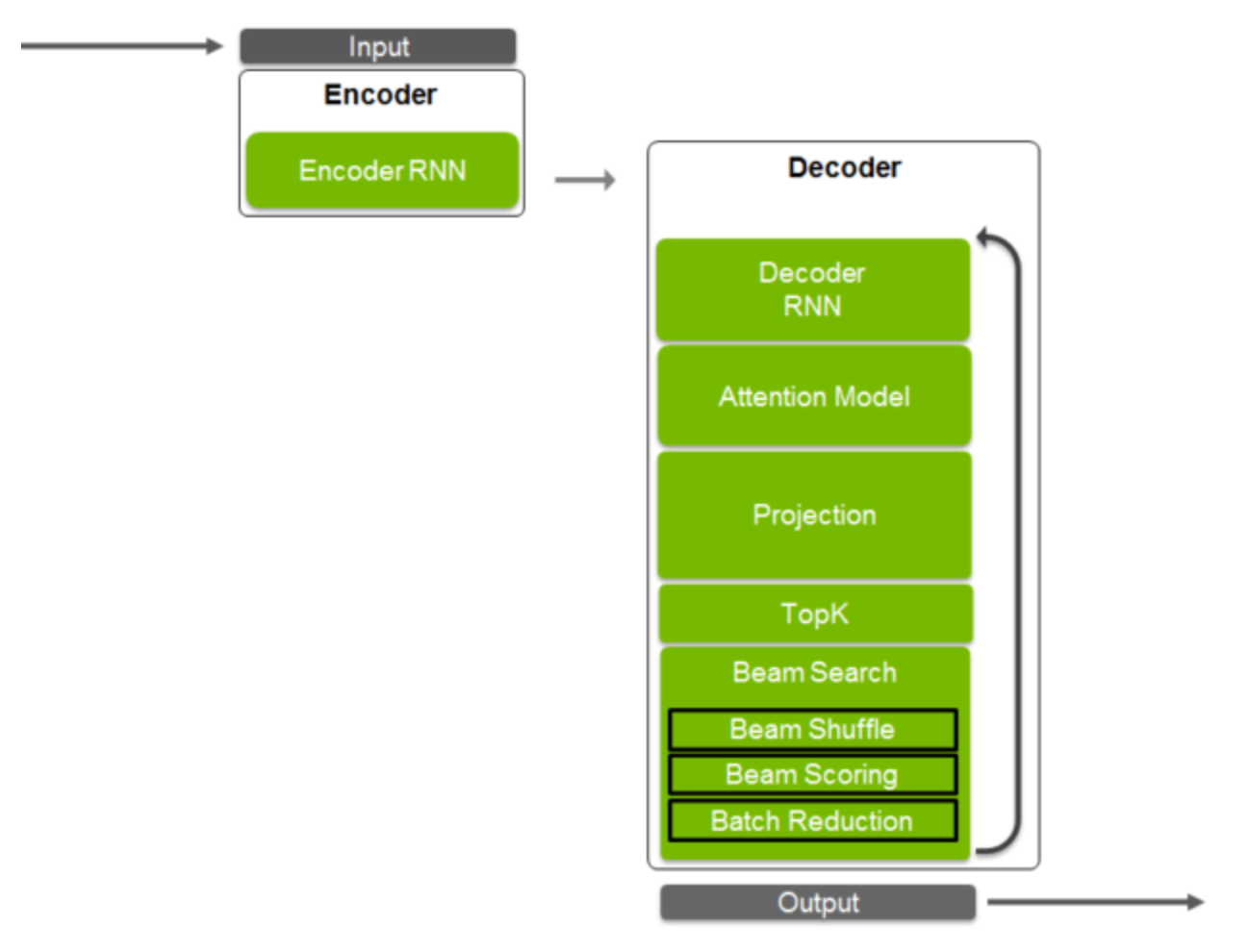
Seq2seq models contain two parts: the encoder and the decoder. The encoder uses a recurrent neural network (RNN) to capture the language-independent “meaning” of the input sequence (phrase, sentence or paragraph) within the state of the system as a fixed-length vector. This approach can be generalized, making it easily transferable to other language pairs. A single state vector captures the meaning of the complete sentence. The decoder takes this state and generates a sequence in the target language. While a comprehensive treatment of NMT layers is beyond the scope of this article, let’s have a quick refresher.
The decoder consists of attention, RNN layers, projection, and beam search. Fig 1 shows the architecture of a seq2seq NMT model; many other variations exist and are used today. The decoder RNN uses the encoder state to generate the target sequence one token at a time. This performs well for short sequences but suffers when the input sequences are long. This happens because the encoder state, a single vector, needs to convey the meaning of all words in the sequence, from the first to the last, which can be quite long if the input sequence is a paragraph.
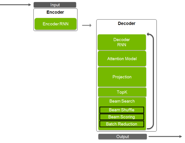
Many languages have structural similarities as well. For example, the first word in an English sentence will likely have a strong influence on the first word chosen in the German translation. These similarities can be used to improve the quality of translations. During the training phase, the encoder RNN is trained to learn the end of the sequence last. It retains information about the more recent training samples, corresponding to the end-of-sentence much more than the information about the beginning of the sequence. This lowers quality of translation since the architecture does not take advantage of the similarity of the structure between languages currently. Attention mechanisms solve this problem by having the decoder focus on specific portions of the input sequence when generating output. The encoder and decoder RNNs pass the output to the attention layer. So far, all tokens are represented by a discrete number from the vocabulary. The discrete output of the attention layer is passed to the projection operation to convert from the discrete space to the continuous space.
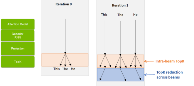
n the continuous space, tokens with similar context are placed close to each other. These projected values compute the probability of all tokens in the vocabulary. Computationally, this would generate a result vector equal to the size of your vocabulary for each vector. This can be extremely memory and computationally expensive for successive operations, so we use the TopK operation. TopK is a partial sorting algorithm that returns K tokens with the highest probability values. These tokens correspond to the most likely characters, words, or subwords from the vocabulary. If K is equal to one, we obtain the most likely token that could be sent back to the decoder RNN to generate the next token, and so on in a loop. The process continues until the end-of-sequence token is generated. The more effective approach is to process multiple, say ‘K’, set of tokens in parallel and then choose the best result in the end. This approach is called a beam search and the number of tokens used, ‘K’, is called token width. Beam search is essentially a directed partial breadth-first tree search algorithm. Let us walk through an example of how this works with a beam width of 3.
The decoder starts with the start-of-sequence tag in the first iteration and predicts 3 tokens as described above. These tokens then get sent as input to the decoder. Each token in turn generates three tokens. So now we would have 32 = 9 tokens. Every subsequent iteration would be a multiple of three. To prevent the inevitable exponential growth, we perform a TopK operation across all the 9 predictions (See Fig 2). Note that this TopK is across all prediction K2 predictions across beams, different from the intra-beam TopK used after a projection operation to pick tokens with the highest probabilities within a beam.
TensorRT 4 introduces new operations and layers used within the decoder such as Constant, Gather, RaggedSoftmax, MatrixMultiply, Shuffle, TopK, and RNN_V2. The TensorRT layers section in the documentation provides a good reference. Let’s now explore a couple of the new layers.
The RaggedSoftMax layer implements cross-channel SoftMax for an input tensor containing sequences of variable lengths. Using an input set with variable length elements differentiates RaggedSoftMax from the older SoftMax layer. Using variable length computations provides more accurate results and faster computations. A second tensor input specifies the sequence lengths to the layer. RNNv2 offers a new API significantly easier to use than the earlier version, RNNv1. RNNv2 adds to the original by implementing recurrent layers such as RNNs, Gated Recurrent Units (GRUs), and Long Short-Term Memory (LSTM). The older RNN layer has been deprecated in favor of this new version but will continue to work to facilitate backward compatibility.
With these new layers, you can now execute complete NMT applications on GPUs to take advantage of optimizations such as kernel fusions, in place concatenations, and reduced precision math for speeding up your application.
Refer to the sampleNMT sample included in the TensorRT samples folder. This modularized sample allows it to serve as a starting point for a larger application. The sample starts from a TensorFlow model checkpoint and covers how to create an attention-based seq2seq type NMT inference engine, import trained weights data, build relevant engines and run inference in TensorRT. This example shows how to use layers such as RNNv2, Constant, MatrixMultiply, Shuffle, RaggedSoftmax, TopK, and Gather.
Neural Collaborative Filtering based Recommender Systems
Neural Collaborative Filtering (NCF) is a common technique powering recommender systems used in a wide array of applications such as online shopping, media streaming applications, social media, and ad placement. Recommender systems suggest items or events for a user as accurately as possible based on past user actions, or characteristics of the user and items. Poor predictions result in low user engagement and potentially lost revenue for enterprises. High response latency makes the application sluggish for interactive applications, resulting in poor user experience. Modern applications employ deep learning-based sophisticated methods, such as NCF, due to their high accuracy. Their ability at learning non-linear relationships between users and items along with powerful generalization capabilities to deal with new users and items enable improved user experiences.
GPUs running TensorRT are well-suited for deploying such deep learning based models for inference, offering near real-time performance in enterprise and hyperscale data centers. TensorRT 4 includes new operations such as Concat, Constant, and TopK plus optimizations for multilayer perceptrons to speed up inference performance of recommendation systems.
Collaborative Filtering is the broad set of techniques that uses past actions of the user, or similar users, to predict future actions. This differs from content-based filtering techniques that use characteristics (tags) associated with users and items to make predictions. One category of traditional collaborative filtering techniques use distance measures such as cosine distance, Pearson coefficients, or K-nearest neighbor to identify users (or items) close to one another, then compute a weighted sum of their ratings to predict the rating for a new user-item pair. The other category of traditional collaborative filtering techniques performs matrix factorization by using singular value decomposition (SVD), principal component analysis (PCA), or probabilistic matrix factorization (PMF).
These methods identify latent features of the users and items, called “embeddings”. The inner dot product of the embeddings can compute their preferences. Let’s say we want to predict the movie rating for a user (“User_A”). We have a matrix capturing ratings by other users, as figure 3 shows. These matrices are generally quite sparse since each user might have rated only a very very small subset of the items (movies in this case) available. Matrix factorization tries to estimate a small set of dense embedding vectors that represent latent factors for users and items which produce ratings in the initial matrix on inner product. This turns the sparse problem into a dense matrix computation and, reduces the dimensionality of the initial problem size by using a small set of latent factors.

However, the performance of matrix factorization techniques can be inhibited by the choice of interaction function, the inner product. In 2017, He et al proposed the use of deep neural networks to model the interaction function between latent factors. This is the core idea behind neural collaborative filtering. NCF can be seen as a generalization of matrix factorization and outperforms its accuracy in many cases.
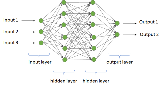
The simplicity of multilayer perceptrons (MLP), plus their strong ability to model nonlinear behaviors, make them an excellent candidate as the neural network architecture in an NCF system. MLPs consist of a fully connected network (FCN), with an input layer, one or more hidden layers, and an output layer, shown in figure 4. Each layer in an MLP layer is an FCN, which means each node connects to every node in the next layer. The inputs to a node get multiplied by weights, added to a bias, and operated on by a non-linear activation function. The user ID for an NCF system is passed as an input, with the network returning the likelihood for all possible events as output. The events with top probabilities are then used to select recommendations.
During implementation, a set of user, context, and item become grouped together for each user-item prediction desired and passed to the MLP as an input as shown in figure 5. The matrix would have five sets of users, context, and items to generate a probability for five user-item pairs. These sets are then concatenated and then passed to the MLP as an input. The output of the MLP is then passed with a TopK layer to select the top recommendations. The layers in TensorRT 4 such as Concat, Constant and TopK enable all operations within an MLP based recommenders to be executed on GPUs during inference. New optimizations further fuse kernel calls to minimize latency and deliver high throughput in functions. Code samples included with the product describe the model structure that triggers these optimizations in more detail.
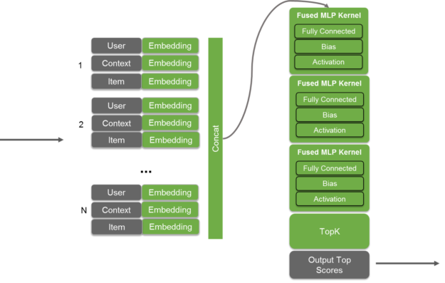
To get started with MLPs, refer to sampleMLP and sampleMovielens code samples. The sample MLP example shows how to create an MLP in TensorRT and trigger the MLP optimization. The sampleMovieLens example shows the complete workflow, from importing the TensorFlow model into TensorRT through the UFF format to building an engine and running inference in TensorRT. The network is trained in TensorFlow on the MovieLens dataset, which contains 6040 users and 3706 movies. Each query to the network consists of a userID and list of MovieIDs. The network predicts the highest-rated movie for each user. This sample also highlights how to use multi-process service (MPS). MPS enables the simultaneous execution of several concurrent inferences on the GPU. Each individual inference, in this case, takes very limited compute resources; running them all concurrently using MPS utilizes the GPU more effectively, resulting in a higher cumulative throughput. Hence it is beneficial to perform inferences in multiple child processes simultaneously. Learn more about MPS in the documentation here.
Speech Recognition Inference with TensorRT
Automatic Speech Recognition (ASR) allows a computer or device to understand spoken words, phrases, and commands. Speech is typically, but not always, transcribed to a written representation. In other cases, more abstract representations encode how the ASR system interprets the meaning of the utterance. Speech recognition can happen locally on personal computing devices such as tablets or phones or in smart devices, automobiles, or robots. Higher accuracy can sometimes be achieved if these edge devices transmit the speech information to an ASR system in the cloud, where larger and more accurate models can be used. Hybrid approaches that augment on-device speech recognition with cloud-based processing are also popular.
Two main approaches to ASR coexist. One involves the use of linguistic models while the other uses deep learning to train a network to map directly from the input sequence to the meaning of the utterance. NVIDIA is working with the open source community to make sure that Kaldi, the leading framework for the linguistic model approach, runs efficiently on GPUs. (Refer to the GTC 2018 Talk Accelerate Your Kaldi Speech Pipeline on the GPU by Hugo Braun to learn ongoing work by NVIDIA in this area). TensorRT can be used to get the best performance from the end-to-end, deep-learning approach to speech recognition. The most noteworthy network for end-to-end speech recognition is Baidu’s Deep Speech 2.
The Deep Speech 2 architecture, shown in figure 6, is actually quite simple. The input for Deep Speech 2 consists of a sequence of 20 ms segments of the input audio signal. Each segment goes into a convolutional stack which extracts features from the audio signal to be used by the rest of the network. The number of layers varies from implementation to implementation, depending on performance vs accuracy requirements, but typically ranges within 3-5 units, including a convolutional layer, a bias layer and a non-linear activation function. The features from this are passed into a stack of 2-5 Gated Recurrent Units (GRU) which remember the context from previous parts of the audio signal and help classify the new bit of sound within that context. Finally, the output of the GRU goes into a 1D-convolution which helps provide look-ahead context. Finally, a fully connected layer is used to project the input from the previous stage into an embedding layer. The result is passed into a TopK which determines the most likely outputs. Finally the most likely outputs are compared with a relatively simple probabilistic linguistic model which regularizes the output. The new layers in TensorRT 4 enable you to maximize the performance of such speech models by deploying optimized implementations for inference on GPUs.
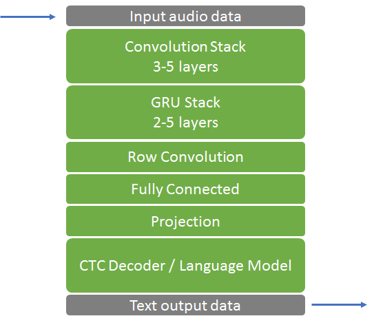
We achieved 60x faster process audio input than was possible with the CPU-only implementation by accelerating all the layers in this model using TensorRT, except the probabilistic language model. With the wide variety of language models (proprietary and open) available today, we are actively working with partners and the community to develop new capabilities in TensorRT that can speed up the ASR pipeline even further.
Support for ONNX format
The Open Neural Network Exchange, or ONNX, is an open format for representing deep learning models. ONNX was introduced to to simplify interchange between frameworks. Leading frameworks such as PyTorch, Caffe2, MxNet, Microsoft Cognitive Toolkit and Chainer participate in the ONNX consortium and support the use of ONNX format within their frameworks. TensorRT 4 includes a native parser for ONNX 1.0 . With this new capability, Developers and data scientists can use the best tools for training their models with this new capability, allowing them take advantage of the optimizations provided by TensorRT that deliver the highest performance possible on GPUs.
You use the NvONNXParser interface with C++ or Python code to import ONNX models. The documentation describes both workflows with code samples. The sample_onnx sample, included with the product, demonstrates use of the ONNX parser with the Python API. It shows how to to import an ONNX model into TensorRT, create an engine with the ONNX parser, and run inference. The code snippet below illustrates how to import an ONNX model with the Python API.
import tensorrt as trt
// Import NvOnnxParser, use config object to pass user args to the parser object
   from tensorrt.parsers import onnxparser
   apex = onnxparser.create_onnxconfig()
// Parse the trained model and generate TensorRT engine
   apex.set_model_file_name("model_file_path")
   apex.set_model_dtype(trt.infer.DataType.FLOAT)
//create the ONNX parser
   trt_parser = onnxparser.create_onnxparser(apex)
   data_type = apex.get_model_dtype()
   onnx_filename = apex.get_model_file_name()
// Generate the TensorRT network after parsing the model file
   trt_parser.parse(onnx_filename, data_type)
// retrieve the network from the parser
   trt_parser.convert_to_trtnetwork()
   trt_network = trt_parser.get_trtnetwork()
The sample provides a number of command line options; use the -h flag to view the full list.
The sampleOnnxMNIST sample demonstrates how to use the ONNX C++ interface to import an MNIST network in ONNX format to TensorRT, build an engine, and run inference. The code snippet below illustrates how to import an ONNX model with the C++ API.
//Create the ONNX parser using SampleConfig object to pass the input arguments
   nvonnxparser::IOnnxConfig* config = nvonnxparser::createONNXConfig();
//Create Parser
   nvonnxparser::IONNXParser* parser = nvonnxparser::createONNXParser(*config);
//Ingest the model
   parser->parse(onnx_filename, DataType::kFLOAT);
//Convert the model to a TensorRT network:
   parser->convertToTRTNetwork();
//Obtain the network from the model:
   nvinfer1::INetworkDefinition* trtNetwork = parser->getTRTNetwork();
The network used in this sample can be found here.
The ONNX parser is an open source project; you can always find the the most up-to-date information regarding the supported operations in Github. See GitHub: ONNX for more information about the ONNX format. You can find a collection of ONNX networks at GitHub: ONNX Models.
TensorFlow – TensorRT Integration
NVIDIA announced the integration of TensorRT with TensorFlow at GTC SV in March 2017. The new integration offers a simple API which applies powerful FP16 and INT8 optimizations using TensorRT from within TensorFlow. TensorRT 3 integration is available for use with TensorFlow 1.8 today from the TensorFlow download site. Our next step is to enable use of TensorRT 4 with the latest version of TensorFlow. The latest integrated version can always be found in the NVIDIA GPU Cloud (NGC) TensorFlow container.
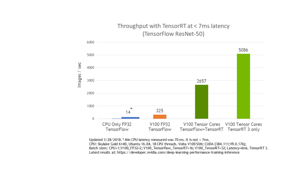
TensorFlow is the most popular deep learning framework today and NVIDIA TensorRT speeds up deep learning inference for all frameworks, including TensorFlow, through optimizations and high-performance runtimes for GPU-based platforms. We wish to give TensorFlow users the highest inference performance possible along with a near transparent workflow using TensorRT. ResNet-50 model performs 8x faster at under 7 ms latency with the TensorFlow-TensorRT integration using NVIDIA Volta Tensor Cores versus running TensorFlow-only on the same GPU, as you can see in figure 7.
Let’s quickly walk through the integrated workflow. TensorFlow integration with TensorRT optimizes and executes compatible sub-graphs, letting TensorFlow execute the remaining graph. While you can still use TensorFlow’s wide and flexible feature set, TensorRT parses the model and applies optimizations to the portions of the graph wherever possible. Your TensorFlow program requires only a couple of new lines of code to facilitate the integration. If you’re currently using TensorRT with TensorFlow models, then you know that applying TensorRT optimizations to TensorFlow models requires exporting the graph. You may need to manually import certain unsupported TensorFlow layers. After freezing the TensorFlow graph for inference in the new workflow, you ask TensorRT to optimize TensorFlow’s sub-graphs. TensorRT then replaces each supported subgraph with a TensorRT optimized node, producing a frozen graph that runs in TensorFlow for inference. Figure 8 illustrates the workflow.
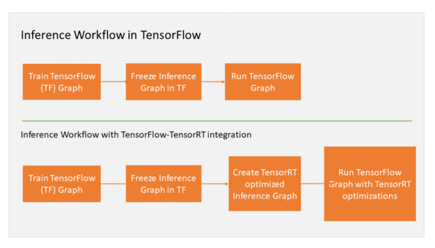
TensorFlow executes the graph for all supported areas and calls TensorRT to execute TensorRT optimized nodes.
Check out more on the integration of TensorRT and TensorFlow in our earlier integration blog post.
Download TensorRT 4 Now!
TensorRT 4 is available for download today from the TensorRT product page. We really enjoy bringing these new features AI developers and are already iterating on new features. While this huge release offers capabilities for many new use cases and applications areas, we continue to push TensorRT forward. We expect to continue growing capabilities across the new application areas in the coming releases. Use the comments section below to tell us how you plan to use the new capabilities in TensorRT 4. If you have issues with TensorRT, check the NVIDIA TensorRT Developer Forum to see if others members of the TensorRT community have a resolution. NVIDIA Registered Developer Program can also file bugs at https://developer.nvidia.com/nvidia-developer-program.
References
[Luong et al 2015] Effective Approaches to Attention-based Neural Machine Translation. Minh-Thang Luong, Hieu Pham, Christopher D. Manning. arXiv:1508.04025
[Villmow 2018] Optimizing NMT with TensorRT. Micah Villmow, GTC 2018
[He et al 2017] Neural Collaborative Filtering. Xiangnan He, Lizi Liao, Hanwang Zhang, Liqiang Nie , Xia Hu, Tat-Seng Chua. arXiv:1708.05031, 2017
[Koehn 2017] Neural Machine Translation. Philipp Koehn. arXiv:1709.07809v1
[Amodei 2015] Deep Speech 2: End-to-End Speech Recognition in English and Mandarin. Baidu Research – Silicon Valley AI Lab. arXiv:1512.02595v1
1 System Specifications: CPU-Only execution in TensorFlow on SKL 6140 18 core, FP32. GPU inference on Tesla V100 running TensorRT 4 RC, FP16; Sorted data, Batch=128, English to German
![]()
