
Large language models (LLMs) are a class of generative AI models built using transformer networks that can recognize, summarize, translate, predict, and generate language using very large datasets. LLMs have the promise of transforming society as we know it, yet training these foundation models is incredibly challenging.
This blog articulates the basic principles behind LLMs, built using transformer networks, spanning model architectures, attention mechanisms, embedding techniques, and foundation model training strategies.
Developers can also explore these training techniques using NVIDIA’s Nemotron family of open models, which provide open weights, data, and full training recipes for reproducing state-of-the-art LLMs.
Model architectures
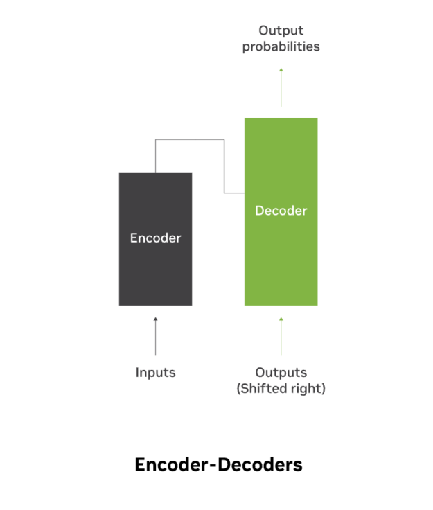
Model architectures define the backbone of transformer networks, broadly dictating the capabilities and limitations of the model. The architecture of an LLM is often called an encoder, decoder, or encoder-decoder model.
Some popular architectures include:
| Architecture | Description | Suitable for |
| Bi-directional Encoder Representation from Transformers (BERT) | Encoder-only architecture, best suited for tasks that can understand language. | Classification and sentiment analysis |
| Generative Pre-trained Transformer (GPT) | Decoder-only architecture suited for generative tasks and fine-tuned with labeled data on discriminative tasks. Given the unidirectional architecture, context only flows forward. The GPT framework helps achieve strong natural language understanding using a single-task-agnostic model through generative pre-training and discriminative fine-tuning. | Textual entailment, sentence similarity, question answering. |
| Text-To-Text Transformer (Sequence-to-Sequence models) | Encoder-decoder architecture. It leverages the transfer learning approach to convert every text-based language problem into a text-to-text format, that is taking text as input and producing the next text as output. With a bidirectional architecture, context flows in both directions. | Translation, Question & Answering, Summarization. |
| Mixture of Experts (MoE) | Model architecture decisions that can be applied to any of the architectures. Designed to scale up model capacity substantially while adding minimal computation overhead, converting dense models into sparse models. The MoE layer consists of many expert models and a sparse gating function. The gates route each input to the top-K (K>=2 or K=1) best experts during inference. | Generalize well across tasks for computational efficiency during inference, with low latency |
Another popular architecture decision is to expand to multimodal models that combine information from multiple modalities or forms of data such as text, images, audio, and video. Although challenging to train, multimodal models offer key benefits of complementary information from different modalities, much as humans understand by analyzing data from multiple senses.
These models contain separate encoders for each modality, like a CNN for images, and transformers for text to extract high-level feature representations from the respective input data. The combination of features extracted from multiple modalities can be a challenge. It can be addressed by fusing features extracted from each modality, or by using attention mechanisms to weigh the contribution of each modality relative to the task.
The joint representation captures interactions between modalities. The model architecture may contain additional decoders for generating task-specific outputs like classifications, caption generation, translation, image generation given prompt text, image editing given prompt text, and the like.
Delving into transformer networks
Within the realm of transformer networks, the process of tokenization assumes a pivotal role in fragmenting text into smaller units known as tokens.
Tokenizers
Tokenization is the first step to building a model, which involves splitting text into smaller units called tokens that become the basic building blocks for LLMs. These extracted tokens are used to build a vocabulary index mapping tokens to numeric IDs, to numerically represent text suitable for deep learning computations. During the encoding process, these numeric tokens are encoded into vectors representing each token’s meaning. During the decoding process, when LLMs perform generation, tokenizers decode the numeric vectors back into readable text sequences.
The process begins with normalization to process lowercase, pruning punctuation and whitespaces, stemming, lemmatization, handling contractions, and removing accents. Once the text is cleaned up, the next step is to segment the text by recognizing word and sentence boundaries. Depending on the boundary, tokenizers can be at word, sub-word, or character-level granularity.
Although word and character-based tokenizers are prevalent, there are challenges with these. Word-based tokenizers lead to a large vocabulary size and words not seen during the tokenizer training process cause many out-of-vocabulary tokens. Character-based tokenizers lead to long sequences and less meaningful individual tokens.
Due to these shortcomings, subword-based tokenizers have gained popularity. The focus of subword tokenization algorithms is to split rare words into smaller, meaningful subwords, based on common character n-grams and patterns. For This technique enables the representation of rare and unseen words via known subwords, resulting in a reduced vocabulary size. During inference, it also handles out-of-vocabulary words effectively reducing vocabulary size, while handling out-of-vocabulary words gracefully during inference.
Popular subword tokenization algorithms include Byte Pair Encoding (BPE), WordPiece, Unigram, and SentencePiece.
- BPE starts with character vocabulary and iteratively merges frequent adjacent character pairs into new vocabulary terms, achieving text compression with faster inference at decoding time by replacing most common words with single tokens.
- WordPiece is similar to BPE in doing merge operations, however, this leverages the probabilistic nature of the language to merge characters to maximize training data likelihood.
- Unigram starts with a large vocabulary, calculates the probability of tokens, and removes tokens based on a loss function until it reaches the desired vocabulary size.
- SentencePiece learns subword units from raw text based on language modeling objectives and uses Unigram or BPE tokenization algorithms to construct the vocabulary.
Attention Mechanisms
As traditional seq-2-seq encoder-decoder language models like Recurrent Neural Networks (RNNs) don’t scale well with the length of the input sequence, the concept of attention was introduced and has proved to be seminal. The attention mechanism enables the decoder to use the most relevant parts of the input sequence weighted by the encoded input sequence, with the most relevant tokens being assigned the highest weight. This concept improves the scaling of input sequence lengths by carefully selecting tokens by importance.
This idea was furthered with self-attention and introduced in 2017 with the transformer model architecture, removing the need for RNNs. Self-attention mechanisms create representations of the input sequence relying on the relationship between different words in the same sequence. By enhancing the information content of an input embedding through the inclusion of input context, self-attention mechanisms play a crucial role in transformer architectures.
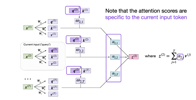
Self-attention is called scaled-dot product attention because of how it achieves context-aware input representation. Each token in the input sequence is used to project itself into Query (Q), Key (K), and Value (V) sequences using their respective weight matrices. The goal is to compute an attention-weighted version of each input token given all the other input tokens as its context. By computing a scaled dotduct of Q and K matrices with relevant pairs determined by the V matrix getting higher weights, the self-attention mechanism finds a suitable vector for each input token (Q) given all key-value pairs that are other tokens in the sequence.
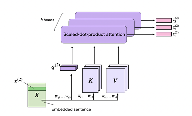
Self-attention further evolved into multi-head attention. The three matrices (Q,K,V) described preceding can be considered as single-head. Multi-head self-attention is when multiple such heads are used. These heads function like multiple kernels in CNNs, attending to different parts of the sequence, focusing on longer-term compared to shorter-term dependencies.
And finally, the concept of cross-attention came about, where instead of a single input sequence as in the case of self-attention, this involves two different input sequences. In the transformer model architecture, that’s one input sequence from the encoder and another processed by the decoder.
FlashAttention
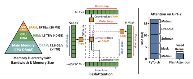
Transformers of a larger size are limited by the memory requirements of the attention layer, which increases in proportion to the length of the sequence. This growth is quadratic. To speed up attention layer computations and reduce its memory footprint, FlashAttention optimizes the naive implementation bottlenecked by repeated reads and writes from slower GPU high bandwidth memory (HBM).
FlashAttention uses classical tiling to load blocks of query, key, and value from GPU HBM (its main memory) to SRAM (its fast cache) for attention computation, and then writes back the output to HBM. It also improves upon memory usage, by not storing large attention matrices from the forward pass; instead relies on recomputing the attention matrix during backprop in SRAM. With these optimizations, FlashAttention brings significant speedup (2-4x) for longer sequences.
Further improved FlashAttention-2 is 2x faster than FlashAttention by adding further optimizations with sequence parallelism, better work partitioning, and reducing non-matmul FLOPs. This newer version also supports multi-query attention as well as grouped-query attention that we describe next.
Multi-Query Attention (MQA)
A variant of attention where multiple heads of query attend to the same head of key and value projections. This reduces the KV cache size and hence the memory bandwidth requirements of incremental decoding. The resulting models support faster autoregressive decoding during inference with minor quality degradation than the baseline multi-head attention architecture.
Group Query Attention (GQA)
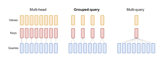
Group-query attention (GQA) is an improvement over MQA to overcome quality degradation issues while retaining the speed-up at inference time. Moreover, models trained using multi-head attention don’t have to be retrained from scratch. They can employ GQA during inference by up-training existing model checkpoints using only 5% of the original training compute. Also, this is a generalization of MQA using an intermediate (more than one, less than number of query heads) number of key-value heads. GQA achieves quality close to baseline multi-head attention with comparable speed to MQA.
Embedding techniques
The order in which words appear in a sentence is important. This information is encoded in LLMs using positional encoding by assigning the order of occurrence of each input token to a 2D positional encoding matrix. Each row of the matrix represents an encoded token of the sequence summed with its positional information. This allows the model to differentiate between words with similar meanings but different positions in the sentence and enables encoding of the relative position of words.
The original transformer architecture combines absolute positional encoding with word embeddings using sinusoidal functions. However, this approach doesn’t allow extrapolation to longer sequences at inference time than those seen during training. Relative position encoding solved this challenge. In this, the content representations for query and key vectors are combined with positional representations that are trainable, relative to the distance between a query and a key that is clipped beyond a certain distance.
RoPE
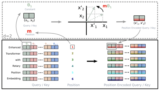
Source:
Rotary Position Embeddings (RoPE) combines the concepts of absolute and relative position embeddings. The absolute position is encoded using a rotation matrix. The relative position dependency is incorporated in self-attention formulation and added to the contextual representation in a multiplicative manner. This technique retains the benefit of sequence length flexibility introduced in the transformer’s sinusoidal position embedding while equipping linear self-attention with relative position encoding. It also introduces decaying inter-token dependency with increasing relative distances, enabling extrapolation to longer sequences at inference time.
AliBi
Transformer-based LLMs don’t scale well to longer sequences due to the quadratic cost of self-attention, which limits the number of tokens of context. Additionally, the sinusoidal position method introduced in the original transformer architecture doesn’t extrapolate to sequences that are longer than it saw during training. This limits the set of real-world use cases where LLMs can be applied. To overcome this, Attention with Linear Biases (ALiBi) was introduced. This technique does not add positional embeddings to word embeddings; instead, it biases query-key attention scores with a penalty that is proportional to their distance.
To facilitate efficient extrapolation for much longer sequences than seen at training time, ALiBi negatively biases attention scores with a linearly decreasing penalty proportional to the distance between the relevant key and query. Compared to sinusoidal models, this method requires no additional runtime or parameters and incurs a negligible (0–0.7%) memory increase. ALiBi’s edge over sinusoidal embeddings is largely explained by its improved avoidance of the early token curse. This method can also achieve further gains by more efficiently exploiting longer context histories.
Training transformer networks
While training LLMs, there are several techniques to improve efficiency and optimize resource usage of underlying hardware configurations. Scaling these massively large AI models with billions of parameters and trillions of tokens comes with huge memory capacity requirements.
To alleviate this requirement, a few methods such as model parallelism and activation recomputation are popular. Model parallelism partitions the model parameters and optimizer states across multiple GPUs so that each GPU stores a subset of the model parameters. It is further classified into tensor and pipeline parallelism.
- Tensor parallelism splits operations across GPUs, often known as intra-layer parallelism focused on parallelizing computation within an operation such as matrix-matrix multiplication. This technique requires additional communication to make sure that the result is correct.
- Pipeline parallelism splits model layers across GPUs, also known as inter-layer parallelization, focused on splitting the model by layers into chunks. Each device computes for its chunk and passes intermediate activations to the next stage. This could lead to bubble time where some devices are engaged in computation and others waiting, leading to a waste of computational resources.
- Sequence parallelism expands upon tensor-level model parallelism by noticing that the regions of a transformer layer that haven’t previously been parallelized and are independent along the sequence dimension. Splitting these layers along the sequence dimension enables distribution of the compute as well as the activation memory for these regions across the tensor parallel devices. Since activations are distributed and have a smaller memory footprint, more activations can be saved for the backward pass.
- Selective activation recomputation goes hand-in-hand with sequence parallelism. It improves cases where memory constraints force the recomputation of some, but not all, of the activations, by noticing that different activations require different numbers of operations to recompute. Instead of checkpointing and recomputing full transformer layers, it’s possible to checkpoint and recompute only parts of each transformer layer that take up a lot of memory but aren’t computationally expensive to recompute.
All techniques add communication or computation overhead. Therefore, finding the configuration that achieves maximum performance and then scaling training with data parallelism is essential for efficient LLM training.
In data parallel training, the dataset is split into several shards, where each shard is allocated to a device. This is equivalent to parallelizing the training process along the batch dimension. Each device will hold a full copy of the model replica and train on the dataset shard allocated. After back-propagation, the gradients of the model will be all-reduced so that the model parameters on different devices can stay synchronized.
A variant of this is called the fully sharded data parallelism (FSDP) technique. It shards model parameters and training data uniformly across data parallel workers, where the computation for each micro-batch of data is local to each GPU worker.
FSDP offers configurable sharding strategies that can be customized to match the physical interconnect topology of the cluster to handle hardware heterogeneity. It can minimize bubbles to overlap communication with computation aggressively through operation reordering and parameter prefetching. And lastly, FSDP optimizes memory usage by restricting the number of blocks allocated for inflight unsharded parameters. Due to these optimizations, FSDP provides support for significantly larger models with near-linear scalability in terms of TFLOPS.
Quantization Aware Training
Quantization is the process in which deep learning models perform all or part of the computation in reduced precision as compared to full precision (floating point) values. This technique enables inference speedups, memory savings, and cost reduction of using deep learning models with minimal accuracy loss.
Quantization Aware Training (QAT) is a method that takes into account the impact of quantization during the training process. The model is trained with quantization-aware operations that mimic the quantization process during training. Models learn how to perform well in quantized representations, leading to improved accuracy compared to post-training quantization. The forward pass quantizes weights and activations to low-precision representations. The backward pass computes gradients using full-precision weights and activations. This enables the model to learn parameters that are robust to quantization errors introduced in the forward pass. The result is a trained model that can be quantized post-training with minimal impact on accuracy.
Train LLMs today
This post covered various model training techniques and when to use them. Check out the post on Mastering LLM Techniques: Customization, to continue your learning journey on the LLM workflow.
Many of the training methods are supported on NVIDIA NeMo, which provides an accelerated workflow for training with 3D parallelism techniques. To get started quickly, clone the NeMo GitHub repositories and follow the Nemotron example configs, which demonstrate best practices for tokenizer setup, parallelism, and training optimization.
