
Deep neural networks (DNNs) are the go-to model for learning functions from data, such as image classifiers or language models. In recent years, deep models have become popular for representing the data samples themselves. For example, a deep model can be trained to represent an image, a 3D object, or a scene, an approach called Implicit Neural Representations. (See also Neural Radiance Fields and Instant NGP). Read on for a few examples of performing operations on a pretrained deep model for both DNNs-that-are-functions and DNNs-that-are-data.
Suppose you have a dataset of 3D objects represented using Implicit Neural Representations (INRs) or Neural Radiance Fields (NeRFs). Very often, you may wish to “edit” the objects to change their geometry or fix errors and abnormalities. For example, to remove a handle of a cup or make all car wheels more symmetric than was reconstructed by the NeRF.
Unfortunately, a major challenge with using INRs and NeRFs is that they must be rendered before editing. Indeed, editing tools rely on rendering the objects and directly fine-tuning the INR or NeRF parameters. See, for example, 3D Neural Sculpting (3DNS): Editing Neural Signed Distance Functions. It would have been much more efficient to change the weights of the NeRF model directly without rendering it back to 3D space.
As a second example, consider a trained image classifier. In some cases, you may want to apply certain transformations to the classifier. For example, you may want to take a classifier trained in snowy weather and make it accurate for sunny images. This is an instance of a domain adaptation problem.
However, unlike traditional domain adaptation approaches, the setting focuses on learning the general operation of mapping a function (classifier) from one domain to another, rather than transferring a specific classifier from the source domain to the target domain.
Neural networks that process other neural networks
The key question our team raises is whether neural networks can learn to perform these operations. We seek a special type of neural network “processor” that can process the weights of other neural networks.
This, in turn, raises the important question of how to design neural networks that can process the weights of other neural networks. The answer to this question is not that simple.
Previous work on processing deep weight spaces
The simplest way to represent the parameters of a deep network is to vectorize all weights (and biases) as a simple flat vector. Then, apply a fully connected network, also known as a multilayer perceptron (MLP).
Several studies have attempted this approach, showing that this method can predict the test performance of input neural networks. See Classifying the Classifier: Dissecting the Weight Space of Neural Networks, Hyper-Representations: Self-Supervised Representation Learning on Neural Network Weights for Model Characteristic Prediction, and Predicting Neural Network Accuracy from Weights.
Unfortunately, this approach has a major shortcoming because the space of neural network weights has a complex structure (explained more fully below). Applying an MLP to a vectorized version of all parameters ignores that structure and, as a result, hurts generalization. This effect is similar to other types of structured inputs, like images. This case works best with a deep network that is not sensitive to small shifts of an input image.
The solution is to use convolutional neural networks. They are designed in a way that is largely “blind” to the shifting of an image and, as a result, can generalize to new shifts that were not observed during training.
Here, we want to design deep architectures that follow the same idea, but instead of taking into account image shifts, we want to design architectures that are not sensitive to other transformations of model weights, as we describe below.
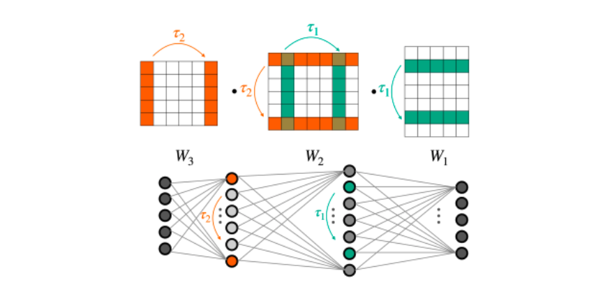
Specifically, a key structural property of neural networks is that their weights can be permuted while they still compute the same function. Figure 2 illustrates this phenomenon. This important property is overlooked when applying a fully connected network to vectorized weights.
Unfortunately, a fully connected network that operates on flat vectors sees all these equivalent representations as different. This makes it much harder for the network to generalize across all such (equivalent) representations.
A brief introduction to symmetries and equivariant architectures
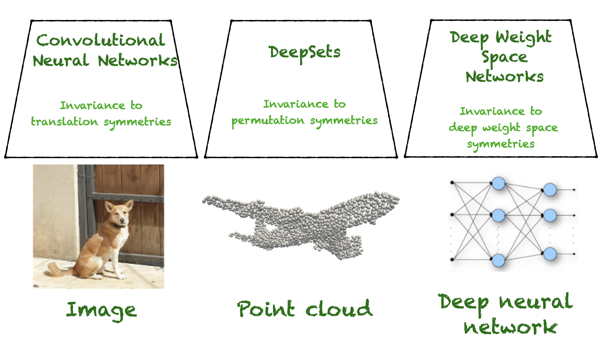
Fortunately, the preceding MLP limitations have been extensively studied in a subfield of machine learning called Geometric Deep Learning (GDL). GDL is about learning objects while being invariant to a group of transformations of these objects, like shifting images or permuting sets. This group of transformations is often called a symmetry group.
In many cases, learning tasks are invariant to these transformations. For example, finding the class of a point cloud should be independent of the order by which points are given the network because that order is irrelevant.
In other cases, like point cloud segmentation, every point in the cloud is assigned a class to which part of the object it belongs to. In these cases, the order of output points must change in the same way if the input is permuted. Such functions, whose output transforms according to the input transformation, are called equivariant functions.
More formally, for a group of transformations G, a function L: V → W is called G-equivariant if it commutes with the group action, namely L(gv) = gL(v) for all v ∈ V, g ∈ G. When L(gv) = L(v) for all g∈ G, L is called an invariant function.
In both cases, invariant and equivariant functions, restricting the hypothesis class is highly effective, and such symmetry-aware architectures offer several advantages due to their meaningful inductive bias. For example, they often have better sample complexity and fewer parameters. In practice, these factors result in significantly better generalization.
Symmetries of weight spaces
This section explains the symmetries of deep weight spaces. One might ask the question: Which transformations can be applied to the weights of MLPs, such that the underlying function represented by the MLP is not changed?
One specific type of transformation, called neuron permutations, is the focus here. Intuitively, when looking at a graph representation of an MLP (such as the one in Figure 2), changing the order of the neurons at a certain intermediate layer does not change the function. Moreover, the reordering procedure can be done independently for each internal layer.
In more formal terms, an MLP can be represented using the following set of equations:
\(f(x)= x_M, \quad x_{m+1}=\sigma(W_{m+1} x_m +b_{m+1}), \quad x_0=x\)
The weight space of this architecture is defined as the (linear) space that contains all concatenations of vectorized weights and biases \([W_m, b_l]_{ m \in [M],l\in[M]}\). Importantly, in this setup, the weight space is the input space to the (soon-to-be-defined) neural networks.
So, what are the symmetries of weight spaces? Reordering the neurons can be formally modeled as an application of a permutation matrix to the output of one layer and an application of the same permutation matrix to the next layer. Formally, a new set of parameters can be defined by the following equations:
\(W_1 \rightarrow P^T W_1\)
\(W_2 \rightarrow W_2P\)
The new set of parameters is different, but it is easy to see that such transformations do not change the function represented by the MLP. This is because the two permutation matrices \(P\) and \(P^T\) cancel each other (assuming an elementwise activation function like ReLU).
More generally, and as stated earlier, a different permutation can be applied to each layer of the MLP independently. This means that the following more general set of transformations will not change the underlying function. Think about these as symmetries of weight spaces.
\((W_1,\dots,W_M) \rightarrow (P_1^TW_1,P_2^TW_2P_1,\dots,P_{M-1}^TW_{M-1}P_{M-2},W_MP_{M-1})\)
Here, \(P_i\) represents permutation matrices. This observation was made more than 30 years ago by Hecht-Nielsen in On the Algebraic Structure of Feedforward Network Weight Spaces. A similar transformation can be applied to the biases of the MLP.
Building Deep Weight Space Networks
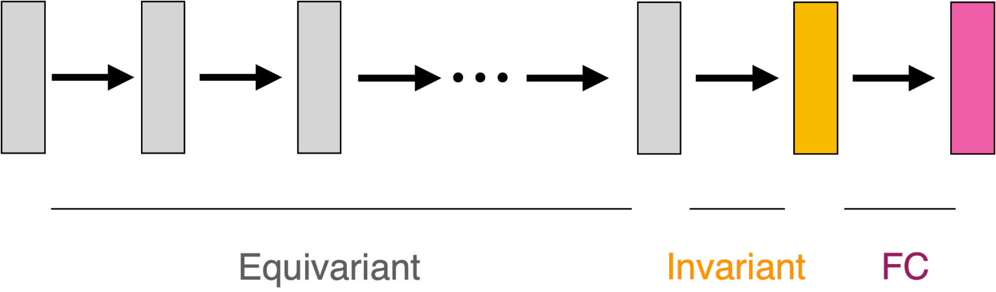
Most equivariant architectures in the literature follow the same recipe: a simple equivariant layer is defined, and the architecture is defined as a composition of such simple layers, possibly with pointwise nonlinearity between them.
A good example of such a construction is CNN architecture. In this case, the simple equivariant layer performs a convolution operation, and the CNN is defined as a composition of multiple convolutions. DeepSets and many GNN architectures follow a similar approach. For more information, see Weisfeiler and Leman Go Neural: Higher-Order Graph Neural Networks and Invariant and Equivariant Graph Networks.
When the task at hand is invariant, it is possible to add an invariant layer on top of the equivariant layers with an MLP, as illustrated in Figure 3.
We follow this recipe in our paper, Equivariant Architectures for Learning in Deep Weight Spaces. Our main goal is to identify simple yet effective equivariant layers for the weight-space symmetries defined above. Unfortunately, characterizing spaces of general equivariant functions can be challenging. As with some previous studies (such as Deep Models of Interactions Across Sets), we aim to characterize the space of all linear equivariant layers.
We have developed a new method to characterize linear equivariant layers that is based on the following observation: the weight space V is a concatenation of simpler spaces that represent each weight matrix V=⊕Wi. (Bias terms are omitted for brevity).
This observation is important, as it enables writing any linear layer \(L:V \rightarrow V\) as a block matrix whose (i,j)-th block is a linear equivariant layer between \(W_j\) and \(W_i\) \(L_{ij} : W_j \rightarrow W_i\). This block structure is illustrated in Figure 4.
But how can we find all instances of \(L_{ij}\)? Our paper lists all the possible cases and shows that some of these layers were already characterized in previous work. For example, \(L_{ii}\) for internal layers was characterized in Deep Models of Interactions Across Sets.
Remarkably, the most general equivariant linear layer in this case is a generalization of the well-known deep sets layer that uses only four parameters. For other layers, we propose parameterizations based on simple equivariant operations such as pooling, broadcasting, and small fully connected layers, and show that they can represent all linear equivariant layers.
Figure 4 shows the structure of L, which is a block matrix between specific weight spaces. Each color represents a different type of layer. \(L_{ii}\) are in red. Each block maps a specific weight matrix to another weight matrix. This mapping is parameterized in a way that relies on the positions of the weight matrices in the network.
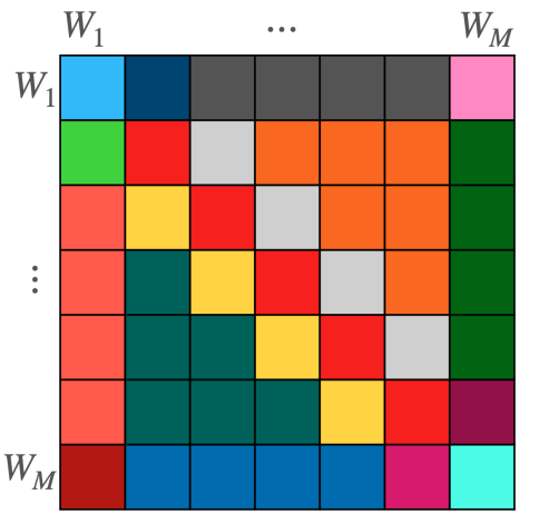
The layer is implemented by computing each block independently and then summing the results for each row. Our paper covers some additional technicalities, like processing the bias terms and supporting multiple input and output features.
We call these layers Deep Weight Space Layers (DWS Layers), and the networks constructed from them Deep Weight Space Networks (DWSNets). We focus here on DWSNets that take MLPs as input. For more details on extensions to CNNs and transformers, see Appendix H in Equivariant Architectures for Learning in Deep Weight Spaces.
The expressive power of Deep Weight Space Networks
Restricting our hypothesis class to a composition of simple equivariant functions may unintentionally impair the expressive power of equivariant networks. This has been widely studied in the graph neural networks literature cited above. Our paper shows that DWSNets can approximate feed-forward operations on input networks—a step toward understanding their expressive power. We then show that DWS networks can approximate certain “nicely behaving” functions defined in the MLP function space.
Experiments
DWSNets are evaluated in two families of tasks. First, taking input networks that represent data, like INRs. Second, taking input networks that represent standard I/O mappings such as image classification.
Experiment 1: INR classification
This setup classifies INRs based on the image they represent. Specifically, it involves training INRs to represent images from MNIST and Fashion-MNIST. The task is to have the DWSNet recognize the image content, like the digit in MNIST, using the weights of these INRs as input. The results show that our DWSNet architecture greatly outperforms the other baselines.
| Method | MNIST INR | Fashion-MNIST INR |
| MLP | 17.55% +- 0.01 | 19.91% +- 0.47 |
| MLP + permutation augmentation | 29.26% +- 0.18 | 22.76% +- 0.13 |
| MLP + alignment | 58.98% +- 0.52 | 47.79% +- 1.03 |
| INR2Vec (architecture) | 23.69% +- 0.10 | 22.33% +- 0.41 |
| Transformer | 26.57% +- 0.18 | 26.97% +- 0.33 |
| DWSNets (ours) | 85.71% +- 0.57 | 67.06% +- 0.29 |
Importantly, classifying INRs to the classes of images they represent is significantly more challenging than classifying the underlying images. An MLP trained on MNIST images can achieve near-perfect test accuracy. However, an MLP trained on MNIST INRs achieves poor results.
Experiment 2: Self-supervised learning on INRs
The goal here is to embed neural networks (specifically, INRs) into a semantic coherent low-dimensional space. This is an important task, as a good low-dimensional representation can be vital for many downstream tasks.
Our data consists of INRs fitted to sine waves of the form a\sin(bx), where a, b are sampled from a uniform distribution on the interval [0,10]. As the data is controlled by these two parameters, the dense representation should extract this underlying structure.
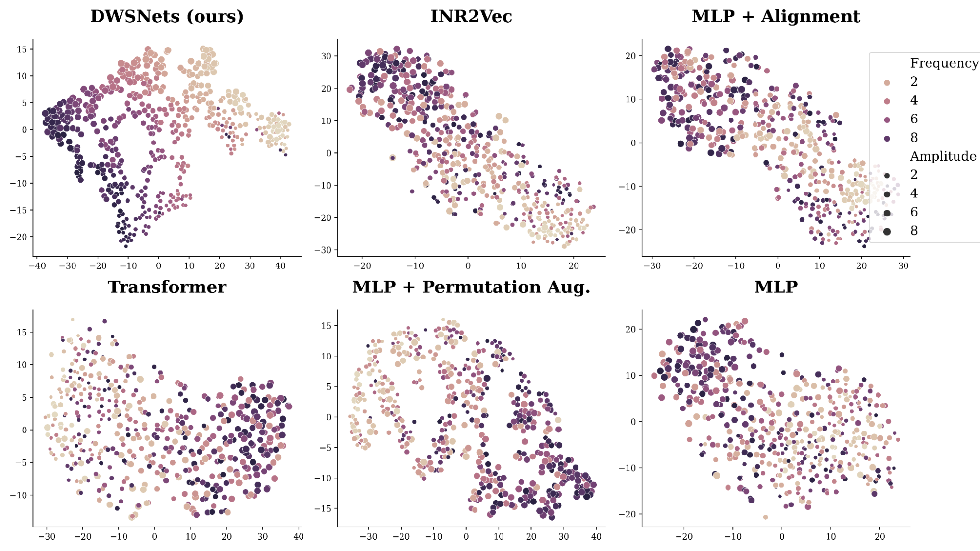
A SimCLR-like training procedure and objective are used to generate random views from each INR by adding Gaussian noise and random masking. Figure 4 presents a 2D TSNE plot of the resulting space. Our method, DWSNet, nicely captures the underlying characteristics of the data while competing approaches struggle.
Experiment 3: Adapting pretrained networks to new domains
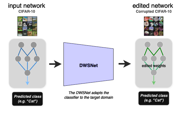
This experiment shows how to adapt a pretrained MLP to a new data distribution without retraining (zero-shot domain adaptation). Given input weights for an image classifier, the task is to transform its weights into a new set of weights that performs well on a new image distribution (the target domain).
At test time, the DWSnet receives a classifier and adapts it to the new domain in a single forward pass. The CIFAR10 dataset is the source domain and a corrupted version of it is the target domain (Figure 6).
The results are presented in Table 2. Note that at test time the model should generalize to unseen image classifiers, as well as unseen images.
| Method | CIFAR10->CIFAR10 corrupted |
| No adaptation | 60.92% +- 0.41 |
| MLP | 64.33% +- 0.36 |
| MLP + permutation augmentation | 64.69% +- 0.56 |
| MLP + alignment | 67.66% +- 0.90 |
| INR2Vec (architecture) | 65.69% +- 0.41 |
| Transformer | 61.37% +- 0.13 |
| DWSNets (ours) | 71.36% +- 0.38 |
Future research directions
The ability to apply learning techniques to deep-weight spaces offers many new research directions. First, finding efficient data augmentation schemes for training functions over weight spaces has the potential to improve DWSNets generalization. Second, it is natural to study how to incorporate permutation symmetries for other types of input architectures and layers, like skip connections or normalization layers. Finally, it would be useful to extend DWSNets to real-world applications like shape deformation and morphing, NeRF editing, and model pruning. Read the full ICML 2023 paper, Equivariant Architectures for Learning in Deep Weight Spaces.
Several papers are closely related to the work presented here, and we encourage interested readers to check them. First, the paper Permutation Equivariant Neural Functionals provides a similar formulation to the problem discussed here but from a different view. A follow-up study, Neural Functional Transformers, suggests using attention mechanisms instead of simple sum/mean aggregations in linear equivariant layers. Finally, the paper Neural Networks Are Graphs! Graph Neural Networks for Equivariant Processing of Neural Networks proposes to model the input neural network as a weighted graph and applying GNNs to process the weight space.
