Why Automatic Augmentation Matters

Deep learning models require hundreds of gigabytes of data to generalize well on unseen samples. Data augmentation helps by increasing the variability of examples in datasets.

The traditional approach to data augmentation dates to statistical learning when the choice of augmentation relied on the domain knowledge, skill, and intuition of the engineers that set up the model training.

Automatic augmentation emerged to reduce the reliance on manual data preprocessing. It combines the idea of applying automated tuning and a random selection of augmentation according to a probability distribution.

Using automatic data augmentation methods such as AutoAugment and RandAugment proved to increase the model’s accuracy through diversifying the samples seen by the model in training. Automatic augmentation makes data preprocessing more complex as each sample in a batch can be processed with a different random augmentation.

In this post, we present how to implement and use GPU-accelerated automatic augmentation to train a model with NVIDIA DALI, using conditional execution.

Automatic data augmentation methods

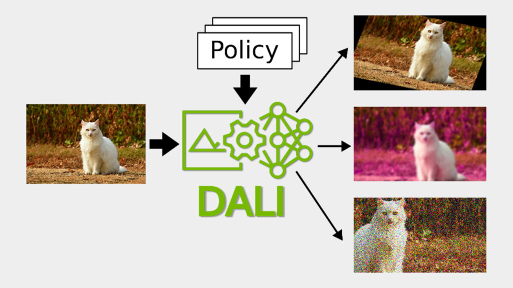
Automatic augmentation is based on standard image transformations like rotation, shearing, blurring, or brightness adjustment. Most operations accept one control parameter called magnitude. The bigger the magnitude, the bigger the impact the operation has on the image.

Traditionally, the augmentation policy is a fixed sequence of operations written by hand by the engineer. What distinguishes automatic augmentation policy from traditional policies is that the choice of augmentation and parameters is not fixed but probabilistic.

AutoAugment employs reinforcement learning to learn the best probabilistic augmentations policy from the data, treating the generalization of the target model as a reward signal. Using AutoAugment, we found new policies for image datasets such as ImageNet, CIFAR-10, and SVHN, beating state-of-the-art accuracies.

The AutoAugment policy is a set of augmentation pairs. Each augmentation is parametrized with a magnitude and probability of applying or skipping the operation. When running the policy, one of the pairs is randomly selected and applied, independently for each sample.

Learning the policy means searching for the best pairs of augmentation, their magnitudes, and probabilities. The target model must be retrained multiple times during the policy search. This makes the computational cost of the policy search immense.

To avoid the computationally costly search step, you can reuse existing policies found on similar tasks. Alternatively, you can use other automatic data augmentation methods that were designed to keep the search step minimal.

RandAugment reduces the policy search step to tuning only two numbers: N and M. N is the number of randomly selected operations to apply in a sequence and M is the magnitude shared by all the operations. Despite RandAugment’s simplicity, we found that this data augmentation method beats the policies found with AutoAugment when used with the same sets of augmentation.

TrivialAgument builds upon RandAugment by removing the two hyperparameters. We proposed applying a single augmentation chosen randomly for each sample. The difference between TrivialAugment and RandAugment is that magnitudes are not fixed but sampled uniformly at random.

The results suggest that a random sampling of augmentations during the training can be more important for model generalization than an extensive search for the carefully tuned policy.

Starting with release 1.24, DALI comes with ready-to-use implementations of AutoAugment, RandAugment, and TrivialAugment. In this post, we show you how to use all these state-of-the-art implementations and discuss the new conditional execution capability in DALI that is the backbone of their implementation.

DALI and conditional execution

Modern GPU architectures significantly speed up deep learning model training. However, to achieve maximum end-to-end performance, batches of data consumed by the model must be preprocessed quickly to avoid bottlenecking on the CPU.

NVIDIA DALI overcomes this preprocessing bottleneck with asynchronous execution, prefetching, specialized loaders, a rich set of batch-oriented augmentations, and integration with popular DL frameworks such as PyTorch, TensorFlow, PaddlePaddle, and MXNet.

To create a data processing pipeline, we combined desired operations in a Python function and decorate the function with @pipeline_def. For performance reasons, the function only defines an execution plan for DALI that is then run asynchronously by DALI executor.

The following code example shows a pipeline definition that loads, decodes, and applies random noise augmentation to the images.

from nvidia.dali import pipeline_def, fn, types 
 
@pipeline_def(batch_size=8, num_threads=4, device_id=0) 
def pipeline(): 
    encoded, _ = fn.readers.file(file_root=data_path, random_shuffle=True) 
    image = fn.decoders.image(encoded, device="mixed") 
    prob = fn.random.uniform(range=[0, 0.15]) 
    distorted = fn.noise.salt_and_pepper(image, prob=prob) 
    return distorted

Eight images distorted with varying levels of salt-and-pepper noise. — *Figure 1. Pipeline output with random noise*

The code of the pipeline is sample-oriented while the output is a batch of images. There is no need for handling batching when specifying operators, as DALI manages that internally.

However, until now, it was not possible to express operations that work on a subset of samples from a batch. This prevented the implementation of automatic augmentation with DALI, as it randomly selects a different operation for each sample.

Conditional execution introduced in DALI enables you to select individual operation for every sample within a batch using regular Python semantics: the if statements. The following code example randomly applies one of two augmentations.

@pipeline_def(batch_size=4, num_threads=4, device_id=0,
              enable_conditionals=True)
def pipeline():
    encoded, _ = fn.readers.file(file_root=data_path, random_shuffle=True)
    image = fn.decoders.image(encoded, device="mixed")
    change_stauration = fn.random.coin_flip(dtype=types.BOOL)
    if change_stauration:
        distorted = fn.saturation(image, saturation=2)
    else:
        edges = fn.laplacian(image, window_size=5)
        distorted = fn.cast_like(0.5 * image + 0.5 * edges, image)
    return distorted

In Figure 2, we increased saturation for some samples and detected the edges with the Laplacian operator in others, based on the fn.random.coin_flip result. DALI translates the if-else statement into an execution plan that splits the batch into two batches according to the if condition. This way, the partial batches are processed separately in parallel, while samples falling into the same if-else branch still benefit from batched CUDA kernels.

Four images, one with sharpened edges and the other three with saturated color. — *Figure 2. Pipeline output with a random choice*

You can easily extend the example to use a random selection of augmentation from an arbitrary set. In the following code example, we defined three augmentations and implemented a select operator that chooses the right one depending on the randomly selected integer.

def edges(image):
    edges = fn.laplacian(image, window_size=5)
    return fn.cast_like(0.5 * image + 0.5 * edges, image)

def rotation(image):
    angle = fn.random.uniform(range=[-45, 45])
    return fn.rotate(image, angle=angle, fill_value=0)

def salt_and_pepper(image):
    return fn.noise.salt_and_pepper(image, prob=0.15)


def select(image, operation_idx, operations, i=0):
    if i >= len(operations):
        return image
    if operation_idx == i:
        return operations[i](image)
    return select(image, operation_idx, operations, i + 1)

In the following code example, we selected a random integer and ran the corresponding operation with the select operator inside the DALI pipeline.

@pipeline_def(batch_size=6, num_threads=4, device_id=0,
              enable_conditionals=True)
def pipeline():
    encoded, _ = fn.readers.file(file_root=data_path, random_shuffle=True)
    image = fn.decoders.image(encoded, device="mixed")
    operations = [edges, rotation, salt_and_pepper]
    operation_idx = fn.random.uniform(values=list(range(len(operations))))
    distorted = select(image, operation_idx, operations)
    return distorted

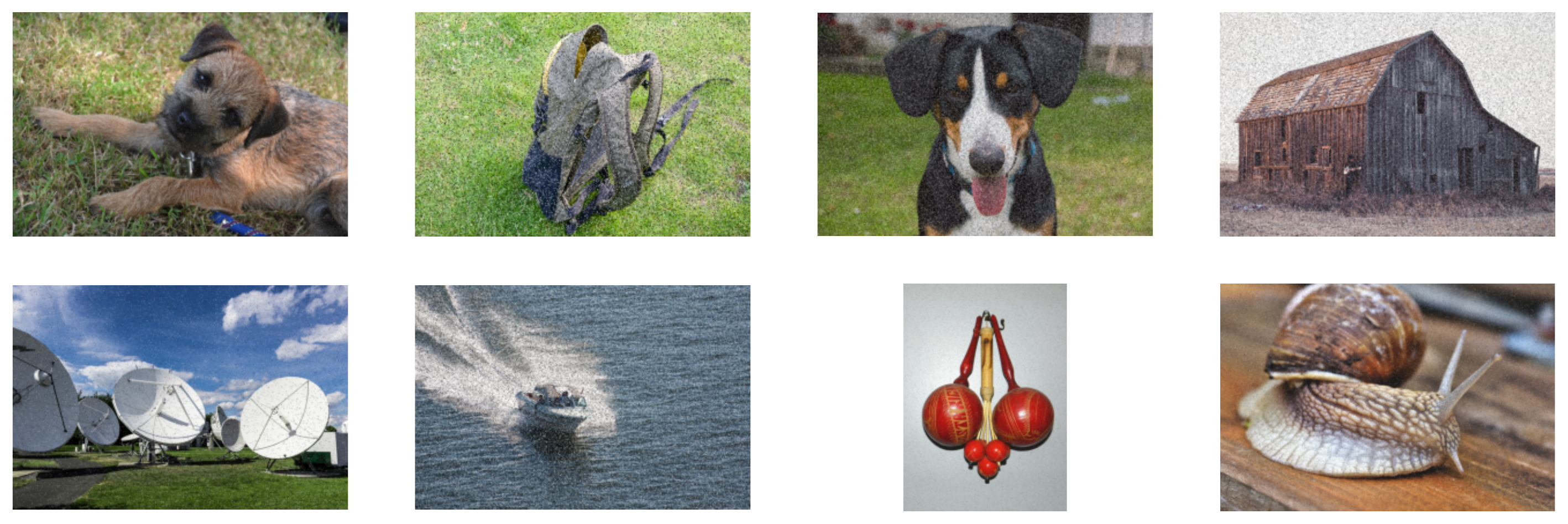
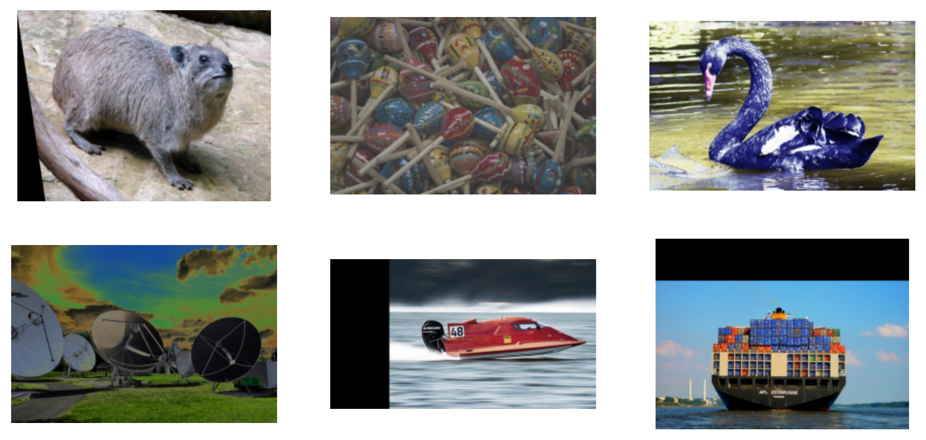
As a result, we got a batch of images where each image is transformed with one randomly selected operation: edge detection, rotation, and salt-and-pepper noise distortion.

Six images: four rotated at different angles, one distorted with salt-and-pepper noise, and one with embossed edges. — *Figure 3. Pipeline output with random augmentations*

In Figure 3, the pipeline applies randomly selected augmentation to each image: rotation, edge detection, or salt-and-pepper distortion.

Automatic augmentation with DALI

With the per-sample selection of operators, you can implement automatic augmentation. For ease of use, NVIDIA introduced the auto_aug module in DALI with ready-to-use implementations of popular automatic augmentations: auto_aug.auto_augment, auto_aug.rand_augment, and auto_aug.trivial_augment. They can be used out-of-the-box or customized by tuning the augmentation magnitudes or building user-defined augmentations of DALI primitives.

The auto_aug.augmentations module in DALI provides a default set of operations shared by the automatic augmentation procedures:

The following code example shows how to run RandAugment.

import nvidia.dali.auto_aug.rand_augment as ra

@pipeline_def(batch_size=6, num_threads=4, device_id=0,
              enable_conditionals=True)
def pipeline():
    encoded, _ = fn.readers.file(file_root=data_path, random_shuffle=True)
    shape = fn.peek_image_shape(encoded)
    image = fn.decoders.image(encoded, device="mixed")
    distorted = ra.rand_augment(image, n=3, m=15, shape=shape, fill_value=0)
    return distorted

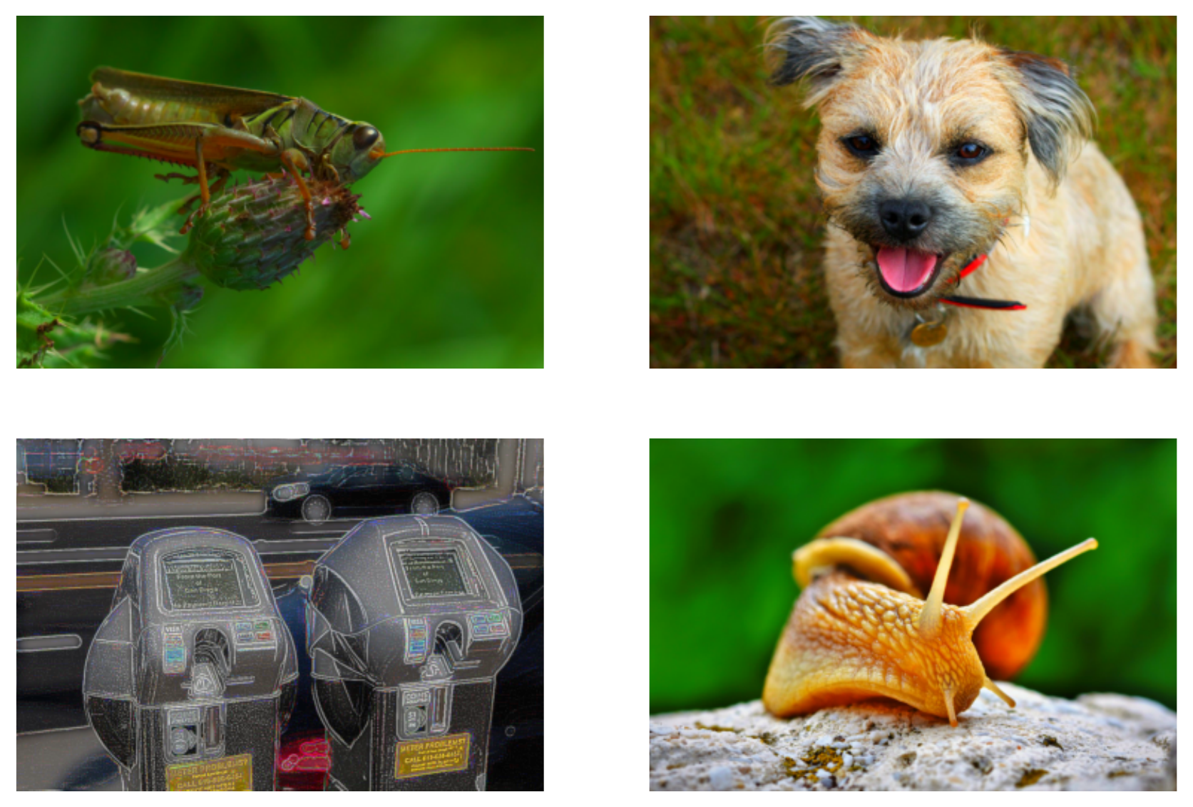
The rand_augment operator accepts the decoded image, the image’s shape, the number of random augmentations to apply in the sequence (n=3), and the magnitude that those operations should have (m=15, out of the customizable [0, 30] range).

Six images with six different distortions. — *Figure 4. Example output of* RandAugment DALI pipeline

The augmentations in Figure 4 fall into two categories: geometric and color transformations.

In some applications, you may have to limit the set of used augmentation. For example, if the dataset consists of pictures of digits, rotating the number “9” by 180 degrees invalidates the associated label. The following code example runs rand_augment with a limited set of augmentations.

from nvidia.dali.auto_aug import augmentations as a

augmentations = [
    a.shear_x.augmentation((0, 0.3), randomly_negate=True),
    a.shear_y.augmentation((0, 0.3), randomly_negate=True),
    a.translate_x.augmentation((0, 0.45), randomly_negate=True),
    a.translate_y.augmentation((0, 0.45), randomly_negate=True),
    a.rotate.augmentation((0, 30), randomly_negate=True),
]

Each augmentation can be parametrized with how the magnitudes map to transformation strength. For example, a.rotate.augmentation((0, 30)) specifies that you want to rotate the image by an angle no bigger than 30 degrees. randomly_negate=True specifies that the angle should be randomly negated, so that you rotate images clock– or counterclockwise randomly.

The following code example applies the augmentations in a manner like RandAugment.

@pipeline_def(batch_size=8, num_threads=4, device_id=0,
              enable_conditionals=True)
def pipeline():
    encoded, _ = fn.readers.file(file_root=data_path, random_shuffle=True)
    shape = fn.peek_image_shape(encoded)
    image = fn.decoders.image(encoded, device="mixed")
    distorted = ra.apply_rand_augment(augmentations, image, n=3, m=15, shape=shape, fill_value=0)
    return distorted

The only difference between the previous two pipeline definitions is that you use a more generic apply_rand_augment operator that accepts additional arguments, the list of augmentations.

Next, add custom augmentation to the set. Use cutout as an example. It randomly covers part of an image with a zeroed rectangle using the DALI fn.erase function. Wrap fn.erase with the @augmentation decorator that describes how the magnitudes will be mapped into cutout rectangles. cutout_size is a tuple of sizes from 0.01 to 0.4 range rather than the plain magnitude.

from nvidia.dali.auto_aug.core import augmentation

def cutout_shape(size):
    # returns the shape of the rectangle
    return [size, size]

@augmentation(mag_range=(0.01, 0.4), mag_to_param=cutout_shape)
def cutout(image, cutout_size, fill_value=None):
    anchor = fn.random.uniform(range=[0, 1], shape=(2,))
    return fn.erase(image, anchor=anchor, shape=cutout_size, normalized=True, centered_anchor=True, fill_value=fill_value)

augmentations += [cutout]

For a change, run the customized set of geometric augmentations like TrivialAugment, that is, with random magnitudes. Changes to the code are minimal; you import and call trivial_augment instead of rand_augment from the aut_aug module.

import nvidia.dali.auto_aug.trivial_augment as ta

@pipeline_def(batch_size=8, num_threads=4, device_id=0,
              enable_conditionals=True)
def pipeline():
    encoded, _ = fn.readers.file(file_root=data_path, random_shuffle=True)
    shape = fn.peek_image_shape(encoded)
    image = fn.decoders.image(encoded, device="mixed")
    distorted = ta.apply_trivial_augment(augmentations, image, shape=shape, fill_value=0)
    return distorted

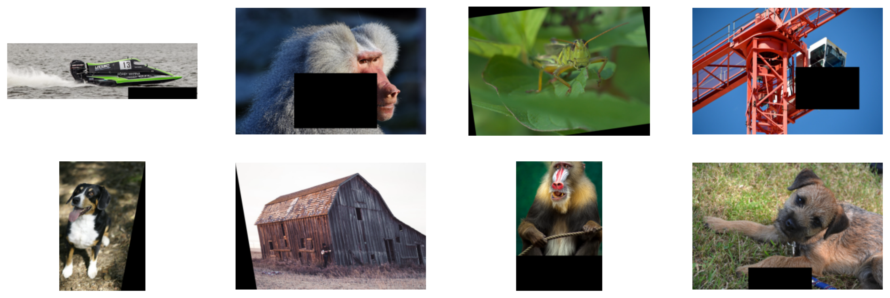
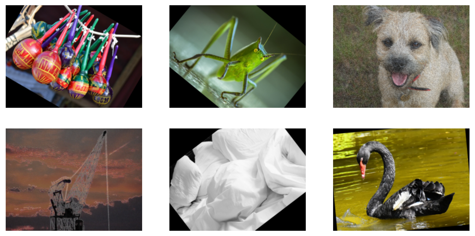
Eight images, each distorted with two random affine transformations. Some of the images are partially overlayed with black rectangles. — *Figure 5. Effects of running* TrivialAugment

Figure 5 shows the effects of running TrivialAugment with the custom set of geometric augmentations and cutouts.

Auto-augmentation performance with DALI

Now, plug DALI and AutoAugment into model training and compare the throughput, using EfficientNet-b0 as an example, adapted from NIVDIA Deep Learning Examples. AutoAugment is a standard part of the preprocessing stage for the models from the EfficientNet family.

In the linked example, the AutoAugment policy is implemented with a PyTorch data loader and runs on a CPU, while the model training happens on a GPU. When the DALI pipeline replaces the data loader running on the CPU, throughput increases. The source code for EfficientNet plus DALI is available in DALI examples.

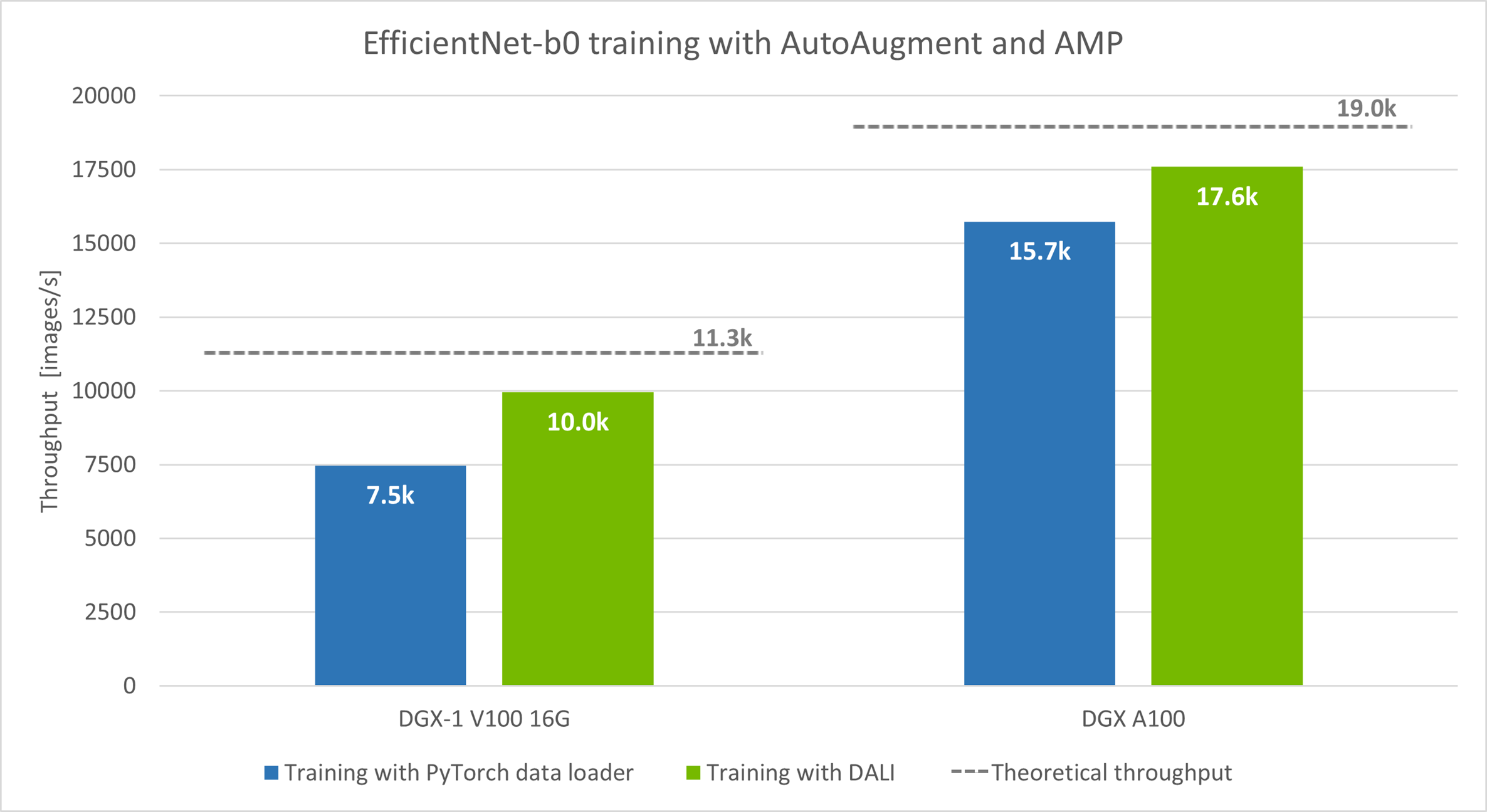
Bar plot comparing EfficientNet training speed with different data loaders: PyTorch CPU data loader, DALI GPU pipeline, and a theoretical speed without data loading. — *Figure 6. EfficientNet-b0 training performance (images/second, the more the better)*

The model ran in automatic mixed-precision mode (AMP), batch sizes: 128 for DGX-1 V100 and 256 for DGX A100.

We ran the experiments with two hardware setups: DGX-1 V100 16 GB and DGX A100. We measured the number of images processed per second (the more the better). In both instances, speed increased: 33% for DGX-1 V100 and 12% for DGX A100.

The theoretical throughput presented with the dashed line in the graph is the upper limit for the training speed that you can expect by improving data preprocessing alone. To measure the theoretical limit, we ran the training with a single batch of synthetic data repeated in every iteration instead of real data. This let us see how fast the model can process batches when no preprocessing is needed.

A significant performance gap between the synthetic case and the CPU data loader case suggests there is a preprocessing bottleneck. To verify the hypothesis, look at the GPU utilization during the training.

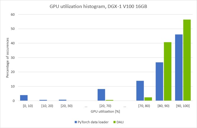
Bar chart compares two variants with different data-preprocessing backends: a CPU PyTorch data loader vs. a GPU DALI pipeline. — *Figure 7. GPU utilization on DGX-1V 16GB increases during EfficientNet-b0 training*

(Batch size 128, automatic mixed-precision mode with DALI data preprocessing)

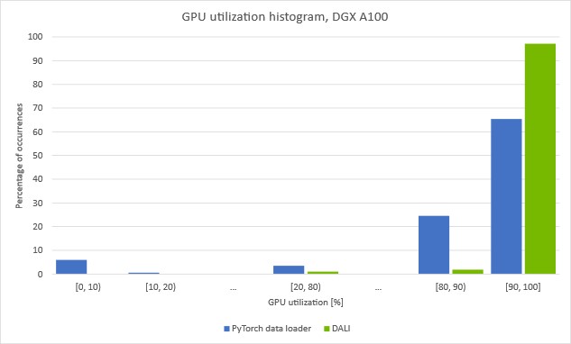
(Batch size 256, automatic mixed-precision mode, with DALI data preprocessing)

The plots show how much time we spent with a given GPU utilization. You can see that when data is preprocessed with a data loader running on the CPU, GPU utilization drops repeatedly. Noticeably, by around 5% of the time, the utilization drops under 10%. This suggests that the training is regularly stalled, waiting for the next batch to arrive from the data loader.

If you move the loading and auto-augmentation step to the GPU with DALI, the [0, 10] bar disappears and the overall GPU utilization increases. The training throughput increase using DALI presented in Figure 6 affirms that we managed to overcome the previous preprocessing bottleneck.

For more information about how to spot and tackle the data-loading bottleneck, see Case Study: ResNet-50 with DALI.