
Efficiency is paramount in industrial manufacturing, where even minor gains can have significant financial implications. According to the American Society of Quality, “Many organizations will have true quality-related costs as high as 15-20% of sales revenue, some going as high as 40% of total operations.” These staggering statistics reveal a stark reality: defects in industrial applications not only jeopardize product quality but also drain a significant portion of a company’s revenue.
But what if companies could reclaim these lost profits and channel them back into innovation and expansion? This is where the potential of AI shines.
This post explores how NVIDIA TAO can be employed to design custom AI models that pinpoint defects in industrial applications, enhancing overall quality.
NVIDIA TAO Toolkit is a low-code AI toolkit built on TensorFlow and PyTorch. It simplifies and accelerates the model training process by abstracting away the complexity of AI models and deep learning frameworks. With the TAO Toolkit, developers can use pretrained models and fine-tune them for specific use cases.
In this post, we leverage an advanced pretrained model for change detection called VisualChangeNet and fine-tune it with the TAO Toolkit to detect defects in the MV Tech Anomaly detection dataset. This comprehensive benchmarking dataset is designed for anomaly detection in machine vision, consisting of various industrial products with both normal and defective samples.
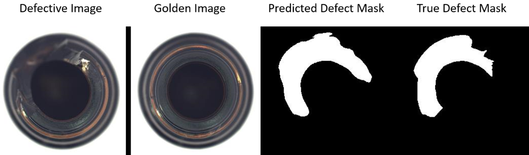
Using the TAO Toolkit, we use transfer learning to train a model that achieves an overall accuracy of 99.67%, 92.3% mIoU, 95.8% mF1, 97.5 mPrecision, and 94.3% mRecall on the bottle class of the MVTec Anomaly dataset. Figure 1 shows the defect mask prediction using the trained model.
Step 1: Setup prerequisites
To follow along with the post and recreate these steps, take the following actions.
- Register for an account on the NGC Catalog and generate your API key by following the steps provided in the NGC User’s Guide.
- Set up the TAO Launcher by following the TAO Quickstart Guide. Download the VisualChangeNet Segmentation Jupyter Notebook for the MVTec dataset. Launch the Jupyter Notebook and run the cells to follow along with this post.
*Note that the VisualChangeNet model works only from the 5.1 version. - Download and prepare the MVTec anomaly detection dataset by following the prompts to the download page and copying the download link for any of the 15 object classes.
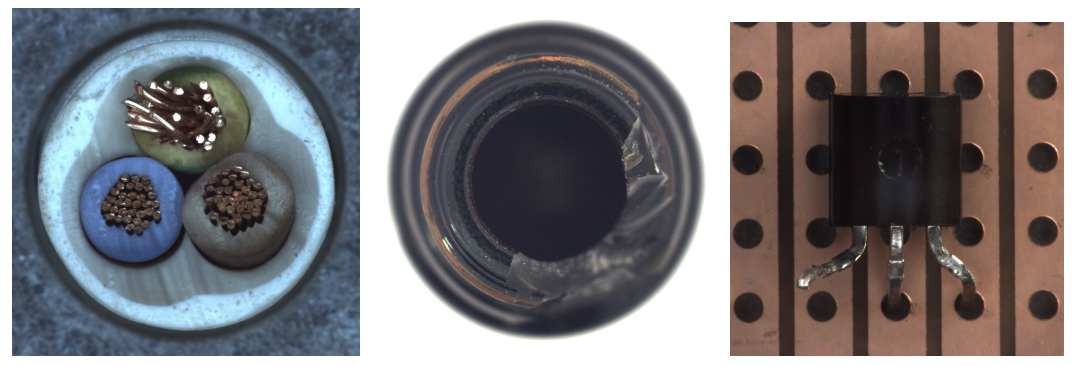
- Paste the download link into the “FIXME” location in section 2.1 of the Jupyter Notebook and run the notebook cell. This post focuses on the bottle object however, all 15 objects work in the notebook. Figure 2 shows the sample defect images in the dataset.
#Download the data
import os
MVTEC_AD_OBJECT_DOWNLOAD_URL = "FIXME"
mvtec_object = MVTEC_AD_OBJECT_DOWNLOAD_URL.split("/")[-1].split(".")[0]
os.environ["URL_DATASET"]=MVTEC_AD_OBJECT_DOWNLOAD_URL
os.environ["MVTEC_OBJECT"]=mvtec_object
!if [ ! -f $HOST_DATA_DIR/$MVTEC_OBJECT.tar.xz ]; then wget $URL_DATASET -O $HOST_DATA_DIR/$MVTEC_OBJECT.tar.xz; else echo "image archive already downloaded"; fi
From MVTec-AD, we leverage the bottle class to showcase automated optical inspection for industrial inspection use cases with VisualChangeNet using the TAO Toolkit.
After the Jupyter Notebook downloads the dataset, run section 2.3 of the notebook to process the dataset into the correct format for VisualChangeNet segmentation.
import random
import shutil
from PIL import Image
os.environ["HOST_DATA_DIR"] = os.path.join(os.environ["LOCAL_PROJECT_DIR"], "data", "changenet")
formatted_dir = f"formatted_{mvtec_object}_dataset"

DATA_DIR = os.environ["HOST_DATA_DIR"]
os.environ["FORMATTED_DATA_DIR"] = formatted_dir

#setup dataset folders in expected format
formatted_path = os.path.join(DATA_DIR, formatted_dir)
a_dir = os.path.join(formatted_path, "A")
b_dir = os.path.join(formatted_path, "B")
label_dir = os.path.join(formatted_path, "label")
list_dir = os.path.join(formatted_path, "list")

#Create the expected folders
os.makedirs(formatted_path, exist_ok=True)
os.makedirs(a_dir, exist_ok=True)
os.makedirs(b_dir, exist_ok=True)
os.makedirs(label_dir, exist_ok=True)
os.makedirs(list_dir, exist_ok=True)
The original dataset was designed for anomaly detection. We merge the two to create a combined dataset of 283 images and then divide them into 253 training set images and 30 testing set images. Both sets include defective samples.
We ensured that the test set included 30% of the defective samples from each defect class, as the ‘bottle’ class predominantly contained ‘no-defect’ images, with around 20 images for each of the three defect classes.
Step 2: Download the VisualChangeNet model
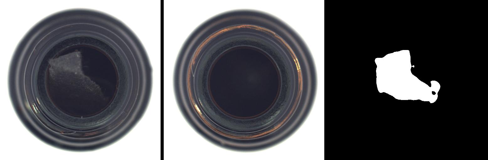
VisualChangeNet model is a state-of-the-art transformer-based change detection model. Central to its design is the Siamese Network. A Siamese Network is a unique neural network architecture composed of two or more identical subnetworks. These “twin” subnetworks accept different inputs but share the same parameters and weights. In the context of VisualChangeNet, this architecture enables the model to compare features between a current image and a reference “golden” image, pinpointing variations and changes. This capability makes Siamese Networks especially adept at tasks like image comparison and anomaly detection.
The model documentation provides more details like architecture and training data. Instead of training a model from scratch, we leverage the pretrained FAN backbone, which was trained on the NV-ImageNet dataset as a starting point. We fine-tune it with the TAO Toolkit on the MVTec-AD dataset for the bottle class.
Run Section 3 of the notebook to install the NGC command-line tool and download the pretrained backbone from NGC.
# Installing NGC CLI on the local machine.
## Download and install
import os
%env CLI=ngccli_cat_linux.zip
!mkdir -p $HOST_RESULTS_DIR/ngccli

# # Remove any previously existing CLI installations
!rm -rf $HOST_RESULTS_DIR/ngccli/*
!wget "https://ngc.nvidia.com/downloads/$CLI" -P $HOST_RESULTS_DIR/ngccli
!unzip -u "$HOST_RESULTS_DIR/ngccli/$CLI" -d $HOST_RESULTS_DIR/ngccli/
!rm $HOST_RESULTS_DIR/ngccli/*.zip
os.environ["PATH"]="{}/ngccli/ngc-cli:{}".format(os.getenv("HOST_RESULTS_DIR", ""), os.getenv("PATH", ""))
!mkdir -p $HOST_RESULTS_DIR/pretrained
!ngc registry model list nvidia/tao/pretrained_fan_classification_nvimagenet*
!ngc registry model download-version "nvidia/tao/pretrained_fan_classification_nvimagenet:fan_base_hybrid_nvimagenet" --dest $HOST_RESULTS_DIR/pretrained
Step 3: Train the model using the TAO Toolkit
In this section, we go into the details of training the VisualChangeNet model using the TAO Toolkit. You can find the details of the Visual ChangeNet models along with the supported pretrained weights in the model card. You can also use the pretrained FAN backbone weights as the starting point for fine-tuning VisualChangeNet, which is what we use to fine-tune on the MVTec-AD dataset.
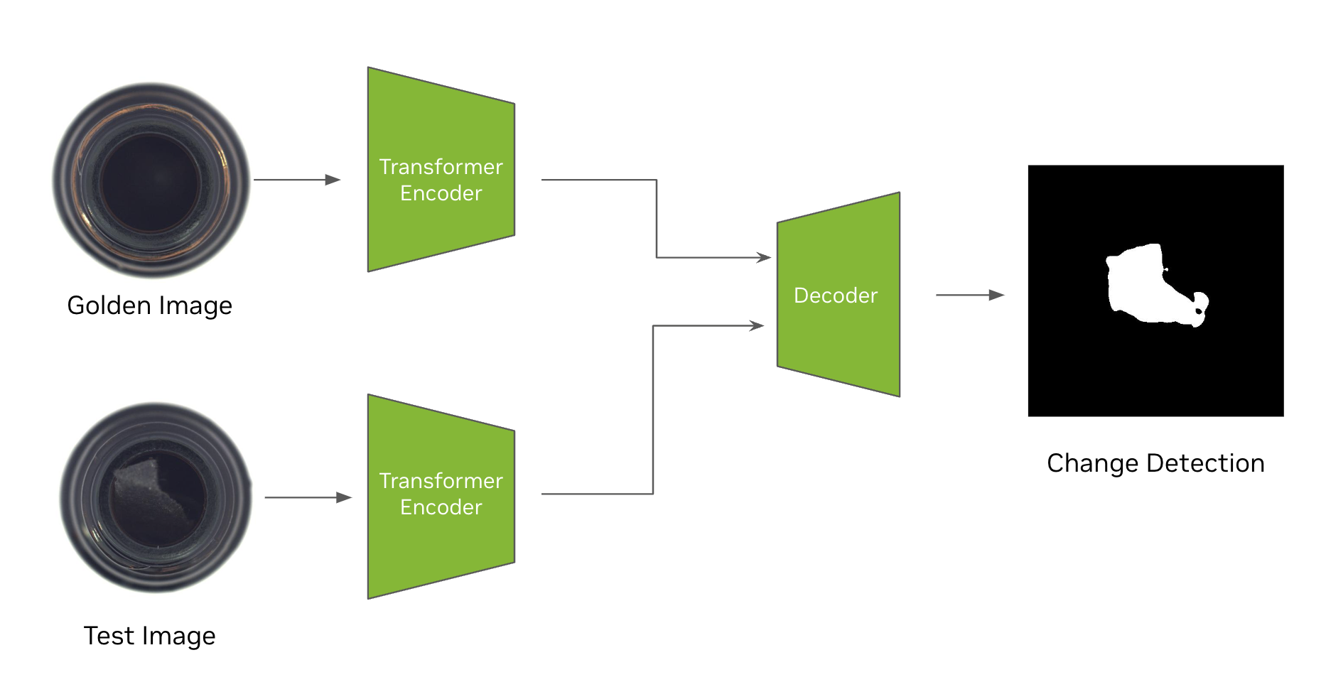
As shown in Figure 4, the training algorithm updates the parameters across all the subnetworks in tandem. In TAO, Visual ChangeNet supports two images as input—a golden sample and a test sample. The goal is to detect a change between the “golden or reference” image and the “test” image. TAO supports the FAN backbone network for Visual ChangeNet architectures.
TAO supports two types of Change Detection networks: Visual ChangeNet-Segmentation and Visual ChangeNet-Classification. In this post, we leverage the Visual ChangeNet-Segmentation model to demonstrate change detection by segmenting the changed pixels between the two input images from the MVTec-AD dataset.
Fine-tuning the VisualChangeNet model is easy with the TAO Toolkit and requires zero coding experience. Simply load the data in the TAO Toolkit, set up the experiment configuration, and run the train command.
The experiment config file defines the hyperparameters for the VisualChangeNet model’s architecture, training, and evaluation. In the Jupyter Notebook, you can view and edit the config file before training the model.
We use this config for fine-tuning the Visual ChangeNet model. In the config, let’s define a Visual ChangeNet model with a pretrained FAN-Hybrid-Base backbone, which is the baseline model. Let’s train the model for 30 epochs with batch size 8. The following section demonstrates a partial experiment config, showing some key parameters. The full experiment config is viewable in the Jupyter Notebook.
encryption_key: tlt_encode
task: segment
train:
  resume_training_checkpoint_path: null
  pretrained_model_path: null
  segment:
    loss: "ce"
    weights: [0.5, 0.5, 0.5, 0.8, 1.0]
  num_epochs: 30
  num_nodes: 1
  val_interval: 1
  checkpoint_interval: 1
  optim:
    lr: 0.0002
    optim: "adamw"
    policy: "linear"
    momentum: 0.9
    weight_decay: 0.01
results_dir: "/results"
model:
  backbone:
    type: "fan_base_16_p4_hybrid"
    pretrained_backbone_path: /results/pretrained/pretrained_fan_classification_nvimagenet_vfan_base_hybrid_nvimagenet/fan_base_hybrid_nvimagenet.pth
Some common values that can be modified to tune the performance of the model are the number of training epochs, the learning rate (lr), the optimizer, and the pretrained backbone. To train from scratch, the pretrained_backbone_path can be set to null, however, this will likely increase the number of epochs and amount of data needed to achieve high accuracy. For more information about the parameters in the experiment config file, see the VisualChangeNet User’s Guide.
Now that the dataset and experiment config is ready, let’s start the training in the TAO Toolkit. Run the code block in section 5.1 to launch a Visual ChangeNet training with a single GPU.
print("Train model")
!tao model visual_changenet train \
                  -e $SPECS_DIR/experiment.yaml \
                    train.num_epochs=$NUM_EPOCHS \
                    dataset.segment.root_dir=$DATA_DIR \
                    model.backbone.pretrained_backbone_path=$BACKBONE_PATH
This cell will begin training the Visual ChangeNet Segmentation model on the MVTec dataset. During training, the model will learn how to identify defective objects and output a segmentation mask showing the defective region. The training log, which includes accuracy on the validation dataset, training loss, learning rate, and trained model, is saved in the results directory set in the experiment config.
Step 4: Evaluate the model
After training is complete, we can use TAO to evaluate the model on a validation dataset. For Visual ChangeNet Segmentation, the output is a segmentation change map for the 2 given input images denoting the pixel-level defects. Section 6 of the notebook will run the command to evaluate the model’s performance.
!tao model visual_changenet evaluate \
                   -e $SPECS_DIR/experiment.yaml \
                    evaluate.checkpoint=$RESULTS_DIR/train/changenet.pth \
                    dataset.segment.root_dir=$DATA_DIR
The evaluate command in TAO will return several KPIs on the validation set such as accuracy, precision, recall, F1 score, and IoU for the defect class (defect pixels).
OA = overall accuracy of change/no change pixels (input dimension – 256×256)
MVTec-AD Binary CD (Bottle Class)
| Model | Backbone | mPrecision | mRecall | mF1 | mIOU | OA |
| VisualChangeNet | FAN-Hybrid-B (pretrained) | 97.5 | 94.3 | 95.8 | 92.3 | 99.67 |
Step 5: Deploy the model
You can use this fine-tuned model and deploy it using NVIDIA DeepStream or NVIDIA Triton. Let’s export it to the .onnx format. Section 8 of the notebook will run the TAO export command.
!tao model visual_changenet export \
                    -e $SPECS_DIR/experiment.yaml \
                        export.checkpoint=$RESULTS_DIR/train/changenet.pth \
                        export.onnx_file=$RESULTS_DIR/export/changenet.onnx
The output .onnx model is saved in the same directory as the trained .pth model. To deploy to Triton, check out the tao-toolkit-triton repository on GitHub. This project provides reference implementations to deploy many TAO models, including Visual ChangeNet Segmentation, to a Triton inference server.
Real-time inference performance
The inference is run on the provided unpruned model at FP16 precision. The inference performance is run using trtexec on embedded Jetson Orin GPUs and data center GPUs. The Jetson devices are running at Max-N configuration for maximum GPU frequency.
Run the following command to run trtexec:
/usr/src/tensorrt/bin/trtexec --onnx=<ONNX path> --minShapes=input0:1x3x512x512,input1:1x3x512x512 --maxShapes=input0:8x3x512x512,input1:8x3x512x512 --optShapes=input0:4x3x512x512,input1:4x3x512x512
--saveEngine=<engine path>
The performance shown here is the inference-only performance. The end-to-end performance with streaming video data might vary depending on other bottlenecks in the hardware and software.
| Platform | Batch Size | FPS |
|---|---|---|
| NVIDIA Jetson Orin Nano 8 GB | 16 | 15.19 |
| NVIDIA Jetson Orin NX 16 GB | 16 | 21.92 |
| NVIDIA Jetson AGX Orin 64 GB | 16 | 55.07 |
| NVIDIA A2 Tensor Core GPU | 16 | 36.02 |
| NVIDIA T4 Tensor Core GPU | 16 | 59.7 |
| NVIDIA L4 Tensor Core GPU | 8 | 131.48 |
| NVIDIA A30 Tensor Core GPU | 16 | 204.12 |
| NVIDIA L40 GPU | 8 | 364 |
| NVIDIA A100 Tensor Core GPU | 32 | 435.18 |
| NVIDIA H100 Tensor Core GPU | 32 | 841.68 |
Summary
In this post, we learned how to use the TAO Toolkit to fine-tune the VisualChangeNet model and use it for segmenting defects in the MVTech dataset, achieving an overall accuracy of 99.67%.
You can also now leverage NVIDIA TAO to detect defects in your manufacturing workflows.
To get started:
- Download the VisualChangeNet model from the NVIDIA NGC catalog.
- Follow the TAO Quickstart Guide to set up the TAO launcher.
- Download the Visual ChangeNet Segmentation Notebook from GitHub
Learn more about the NVIDIA TAO Toolkit from NVIDIA Docs.
