Adversarial training (also called GAN for Generative Adversarial Networks), and the variations that are now being proposed, is the most interesting idea in the last 10 years in ML, in my opinion.
– Yann LeCun, 2016 [1].
You heard it from the Deep Learning guru: Generative Adversarial Networks [2] are a very hot topic in Machine Learning. In this post I will explore various ways of using a GAN to create previously unseen images. I provide source code in Tensorflow and a modified version of DIGITS that you are free to use if you wish to try it out yourself.
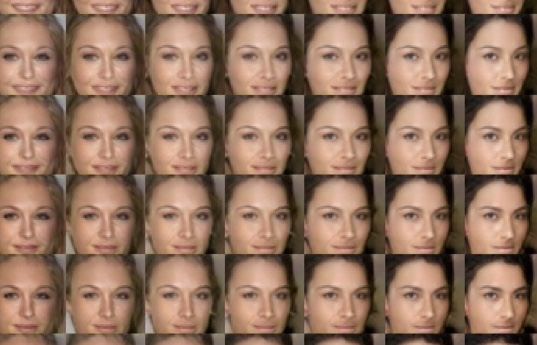
Figure 1 gives a preview of what you will learn to do in this series of posts. Part 1 will give you an understanding of GANs and part 2 applies GAN models to generating celebrity face images.


What is a Generative Model?
In machine learning, a generative model learns to generate samples that have a high probability of being real samples like the samples from the training dataset. Let’s take an example to understand what this means: consider a world composed of all possible 64×64 8-bit RGB images. There are 23x8x64x64 possible arrangements of the pixel values in those images. This is a staggering number, much greater than the number of particles in the universe. Now consider the set of images that represent faces of people. Even though there are many, they represent a tiny fraction of all the images in the world. Learning a probability distribution of the set of face images means that the model needs to learn to assign a high probability (of being a real sample) to the images that represent a face and a low probability to other images.
Finally, consider a dataset of a few thousand face images: learning to generate new samples from this dataset means that the model needs to learn the distribution from which the images in the dataset were drawn. Ultimately the model should be able to assign the right probability to any image—even those that are not in the dataset. A generative face model should be able to generate images from the full set of face images.
How Do Generative Adversarial Networks Work?
The typical GAN setup comprises two agents:
- a Generator G that produces samples, and
- a Discriminator D that receives samples from both G and the dataset.
G and D have competing goals (hence the term “adversarial” in Generative Adversarial Networks): D must learn to distinguish between its two sources while G must learn to make D believe that the samples it generates are from the dataset.
A commonly used analogy for GANs is that of a forger (G) that must learn to manufacture counterfeit goods and an expert (D) trying to identify them as such. But in this case—and this is a very important GAN feature— forgers have insider information into the police department: they have ways to know when and why their products are marked as fake (though they never get to see any of the real goods). Likewise, the police have access to a “higher authority” that lets them know whether their guesses are correct. During training G and D keep playing this game, getting better as they play, until they both become so good that the samples produced by G are indistinguishable from the real stuff.
A Generative Adversarial Play
Let me illustrate with an example: suppose I train a GAN on a dataset of luxury handbags. The following dialogue would be a plausible play.
The Expert stands in a room in front of the Higher Authority. The Forger is lurking in the background and can hear anything The Expert says, though he cannot see any of the action. The Higher Authority picks a luxury handbag from a drawer and presents it to The Expert. The low, resonating voice of the Higher Authority echoes through the room.
Higher Authority: Is this a luxury handbag?
Expert: Hmmm, I can’t say I’ve ever seen a luxury handbag before. This looks fine enough but I know for a fact that The Forger would be trying to deceive me so I say it’s a fake.
Higher Authority: Wrong! That is a fine luxury handbag.
The Higher Authority now requests a sample from The Forger, who produces a carrot. The carrot is presented to The Expert.
Higher Authority: Is this a luxury handbag?
Expert: Well that does look different from the previous thing but I’ve been a bit too prudent before so I say it’s a luxury handbag! [A faint snickering noise is heard from the direction of The Forger.]
Higher Authority: Wrong again! It’s a fake. [The Expert grumbles.]
The Higher Authority picks another luxury handbag from a drawer and presents it to The Expert.
Higher Authority: Is this a luxury handbag?
Expert: OK, that does share some resemblance with the bag I’ve seen before and it’s definitely unlike the other orange cone so I say it’s a luxury handbag! [The Expert holds his breath.]
Higher Authority: Correct. [The Expert sighs.]
[The Higher Authority now requests a sample from The Forger, who produces a slightly different carrot. The Higher Authority shows signs of discontent.]
Higher Authority: OK, is this a luxury handbag?
Expert: Why, you’ve got to be kidding! That’s the same fake you showed me before! You can’t put anything in it. It’s definitely a fake!
[The Higher Authority decides to give The Forger another chance. Elated, The Forger runs to his vault and comes back with a wallet.]
Higher Authority: Is this a luxury handbag?
Expert: Apparently you can shove stuff in it, like the other handbags so I say it’s a luxury handbag!
Higher Authority: Ha! Wrong again!
[The Higher Authority picks another luxury handbag from the drawer and presents it to The Expert.]
Higher Authority: Is this a luxury handbag?
Expert: I have no idea. I don’t want to commit. 50/50?
[A droplet of sweat emerges from The Expert’s forehead.]
Higher Authority: This is a 100% luxury handbag!
[The Higher Authority now requests a sample from The Forger. The Forger runs to his vault and comes back with another wallet.]
Higher Authority: Is this a luxury handbag?
Expert: This doesn’t have handles! It’s a fake!
[The Higher Authority, feeling generous, gives The Forger another chance. The Forger runs to the nearest store and hastily comes back with a plastic bag].
Higher Authority: Is this a luxury handbag?
Expert: Mmm, it’s got handles and you can put stuff in it. Is this real?
Higher Authority: Wrong!
The Expert: OK I get it. The luxury bags had leathery bits. And a shiny logo. I’ll be more careful next time! I can feel I’m getting good at this!
I will spare you further details of this fascinating story but in the end the forger learns to produce the most sophisticated designer handbags that even a cohort of experts would not be able to identify as fakes (better than random guessing).
GAN Behavior in More Detail
One important aspect to keep in mind here is the fact that since D is trained continuously, G cannot simply go about generating the same samples over and over. In particular, if D has ample capacity, it may be able to memorize all the samples that G ever produced and become expert at spotting fakes. How would G then be able to continuously handcraft novel samples? Going back to our dataset of face images, assuming your are G and already in possession of a few realistic images (or at least deemed as such by D), one reasonable way of coming up with an increasing number of realistic images would be to apply small perturbations to the images that you already have: crops, rotations, color transformations, etc. This way you could create a virtually infinite number of new images, but chances are D would start noticing patterns there and punish you.
In order to alleviate this issue, G learns to generate very different samples: given a set of random numbers, which is called the latent representation, or in short the z vector, and through a number of neural layers, G learns to generate new samples that depend on z sufficiently strongly that a different z will yield a very different sample.
It may be hard to believe at first, but through training, every factor in z, or combination thereof, specializes toward one characteristic feature of the dataset. For example, in a dataset of face images, factors might represent the gender of the person, the color of their skin, their pose, etc.
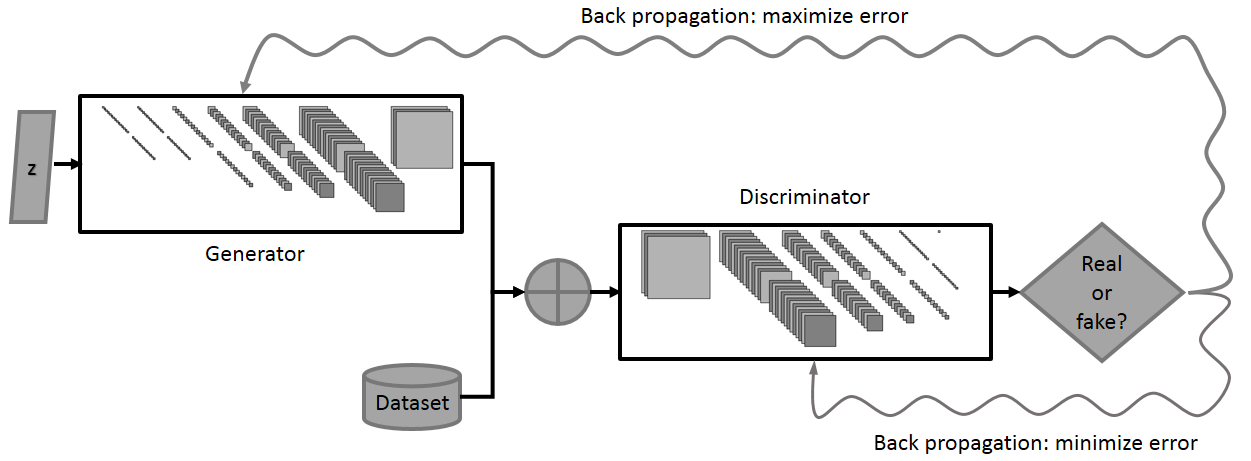
Figure 2 summarises the GAN framework. Although there exist variations of the original training schedule, training is usually a three-stage process in which:
- D receives an image from the dataset and is optimized to classify it as “real”. In practice, this means that its parameters are updated through gradient descent in a direction that moves it closer to classifying the image as real (probability one).
- A random z is drawn from which G generates a new sample. D receives the sample and is optimized to classify it as “fake” (probability zero).
- G is optimized to make D classify the sample as “real” .
Why Are GANs So Popular?
GANs are popular partly because they tackle the important unsolved challenge of unsupervised learning, and partly because the amount of available unlabelled data is considerably larger than the amount of labelled data. I can’t resist another quote from our esteemed Deep Learning luminary:
If intelligence was a cake, unsupervised learning would be the cake, supervised learning would be the icing on the cake, and reinforcement learning would be the cherry on the cake. We know how to make the icing and the cherry, but we don’t know how to make the cake. – Yann LeCun, 2016.
Another reason for their popularity is that GANs are considered to generate the most realistic images among generative models [2]. This is subjective, but it is an opinion shared by most practitioners.
Besides, the learned latent representation in a GAN is often very expressive: arithmetic operations in the latent space, that is to say the space of the z vectors, translate into corresponding operations in feature space. For example, you can see in Figure 1 that if you take the representation of a blond woman in latent space, subtract the “blond hair” vector and add back the “black hair” vector, you end up with a picture of a woman with black hair in feature space. That is truly amazing.
Generating Images of Hand-Written Numbers

An introduction to any deep learning topic would be incomplete without an application to the MNIST [4] dataset, a popular dataset featuring images of handwritten digits (Figure 3).
Network Topology
Note that labels aren’t required to train a GAN, but if I do have labels (as is the case for MNIST) I can use them to train a conditional GAN. A conditional GAN is one that is conditioned to generate and discriminate samples based on a set of arbitrarily chosen attributes. On MNIST, I can condition the GAN on the class of the number I would like to generate. In practice, I concatenate a one-hot representation of the class to the activations of every layer. For fully-connected layers the one-hot representation is just a vector of length 10 (because we have 10 classes of digits) with zeros everywhere except when the index matches the class ID. This idea can be extended to convolutional layers too: in this case conditioning is materialized by a set of 10 feature maps with zeros everywhere except for the feature map whose index is the class ID, which is filled with ones. During training, the latent representation z is sampled from a 100-dimensional normal distribution; an arbitrary choice that yields acceptable results.
Network conditioning, and the topologies of my G and D networks (a slightly modified version of DCGAN [5]) are illustrated in Figure 4. Activation functions are not shown in this figure, but importantly the activation function for the last layer in D is a typical sigmoid.
![Figure 4: Top: the generator (G) network. Bottom: the discriminator (D) network. Layers are traversed from left to right. Network conditioning is illustrated by the black (zeros) and white (ones) feature maps/units. In the above example the third feature map is white, denoting the fact that the corresponding label is assigned to the third class (digit “3”). Implementation based on [6]. Grey feature maps/units mark computed activations.](https://developer.nvidia.com/blog/parallelforall/wp-content/uploads/2017/04/figure4.png)
discriminator_1) which receives images from G.

One technicality is that in order to create two identical instances of D I need to create the layers twice and let Tensorflow know that I want to reuse variables (weights and biases). This is easily done with a call to scope.reuse_variables() as in the following example code.
# call this function again with reuse=True to create a clone of the discriminator
def discriminator(self, image, y=None, reuse=False):
    with tf.variable_scope("discriminator") as scope:
        if reuse:
            scope.reuse_variables()
        # define your variables and ops here
Another important aspect to keep in mind is the set of parameters passed to the optimizer. By default, Tensorflow optimizers (subclasses of tf.train.Optimizer) compute gradients with respect to all trainable variables in the graph and update them all on every iteration of the optimization loop. That is not what you want in the GAN framework: when you train D to identify generated samples, you really only want to modify the state of D. If you let the optimizer change all variables including those of G then it would be just as easy to make G generate garbage and that would not be a fair play. So when you train D you want to freeze the state of G and vice versa. That might sound obvious but since it took me a while to figure it out, I thought I would mention it. Again, this is easily done in Tensorflow with optional parameters (in bold letters in the following) to the optimizer.
vars = tf.trainable_variables()
g_vars = [var for var in vars if 'g_' in var.name]
grads = optimizer.compute_gradients(g_loss, var_list=g_vars)
Objective Functions
D is trained to predict a probability distribution: the probability that a sample $latex x$ belongs to each of the known classes. There are only two classes since a sample is either real or fake. In the original formulation of GAN, D is trained to maximise the probability of guessing the correct label by minimizing the corresponding cross-entropy loss \(L=-\sum_i p_i log(q_i)\), where \(p\) is a one-hot encoding of the label, \(q\) is the predicted probability distribution and \(i\) is the class index. If \(D(x)\) represents the probability that \(x\) is a data sample, then \(L=-log(1-D(G(z))\) for generated samples.
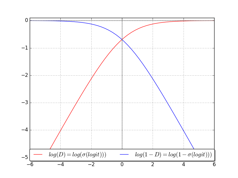
When the GAN framework is formulated as a minimax game, D tries to minimize \(L\) and G tries to maximise it. That’s rather unfortunate for G because during the early phases of training when the output of G is less than convincing, D easily assigns a very low probability to \(G(z)\). This implies that the number \(x\) before the last sigmoid \(\sigma(x)=1/{1+e^-x}\) activation function in D is a large negative number and, as the blue curve in Figure 6 shows, the loss saturates (it is flat and the gradient is tiny) as highlighted in [2].
This makes G learn very slowly, if at all. Therefore it’s common to reformulate the optimization objective for G as a maximisation of \(L=log(D(G(z))\)—the red curve—instead, which yields the same solution but exhibits much stronger gradients in the negative quadrant. Another common solution is to flip the labels: make D predict 1 when optimizing for G. One further refinement that I implemented to alleviate the penalty of an overconfident D is to use one-sided label smoothing and replace the hard label of 1 when optimizing D on real samples with a softer 0.9, as suggested in [2].
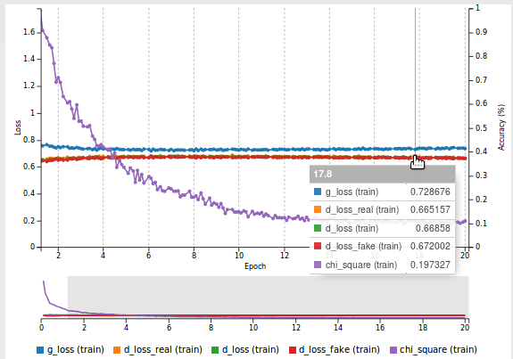
The first thing that I usually check when training a neural network is whether the loss function is going down. However here there are two components of the total loss: D’s loss and G’s loss. By construction, the two losses cannot simultaneously go down. Otherwise D and G wouldn’t be called adversaries! How do you determine whether training is successful? This turns out to be rather difficult in practice, and the subject of ongoing research.
For one thing, you can check whether the game is well balanced. How does that translate into meaningful loss values? If G’s loss is very low this means D is unable to recognize fake samples, possibly because it classifies everything as real. Remember that all the knowledge in G comes from D through back-propagation. G is therefore unlikely to generate good samples if D is doing a poor job at spotting fakes. At equilibrium you would expect D to not be able to do better than random guessing, meaning that it would assign probability 50% to all samples. Going back to the definition of the cross-entropy loss, this would yield a loss value of $latex -log(0.5)=69%$. That number should be easy enough to remember.
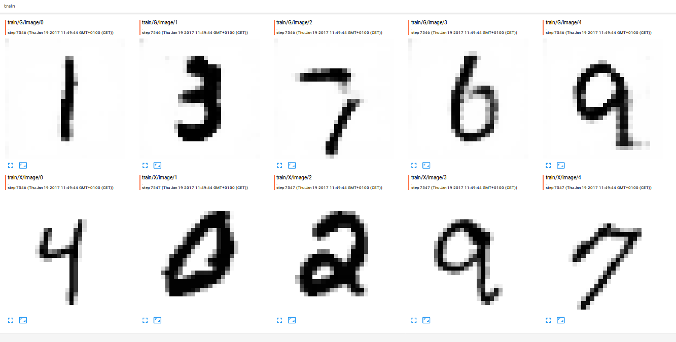
A well balanced game means that both players are equally good… or bad! How do you figure out how well players are doing? One solution is to stare at the generated samples. That is probably what most people do and admittedly I have engaged in a fair amount of staring myself. Tensorflow makes it easy to visualize generated samples by adding a variable to the collection of Tensorboard summaries:
tf.summary.image("G",G))
This causes generated images to be added periodically to my Tensorboard log and I can then monitor them in real time as illustrated on Figure 7.
Since it is not practical to keep looking at the generated samples, I implemented the following metric: remember that G is learning to approximate the probability distribution of the world from which our dataset samples are drawn. One simple proxy that I can use here is to compare the unconditional (non-spatial) distributions of the real and generated samples respectively. For every batch, I calculate histograms of pixel values from each source and compare them using the \(\chi^2\) distance operator. A low \(\chi^2\) value, though not sufficient, is necessary for a good approximation of the data distribution and this metric is easy to implement:
value_range = [0.0, 1.0]
nbins = 100
hist_g = tf.histogram_fixed_width(self.G, value_range, nbins=nbins, dtype=tf.float32) / nbins
hist_x = tf.histogram_fixed_width(self.images, value_range, nbins=nbins, dtype=tf.float32) / nbins
chi_square = tf.reduce_mean(tf.div(tf.square(hist_g - hist_x), hist_g + hist_x))
tf.summary.scalar("chi_square", chi_square))
Figure 8 shows the loss curve in DIGITS. As you can see, all losses are relatively close to 69%, an indication of a well balanced game. Also, the \(\chi^2\) curve (purple) goes down steadily, another reassuring sign.
Sampling
I could pick random values of z and generate random images but it would be great if I could more deterministically choose attributes of the images I create. Remember that in my conditional GAN, the latent representation (z) and the class labels are separate. Therefore, I can pick one value of z and generate matching images for all classes. I can also do what I call a class sweep: pick one z and slowly interpolate across classes to get smooth transitions between digits. Have a look at Figure 9 for examples. Each grid uses the same value of z and a different label.
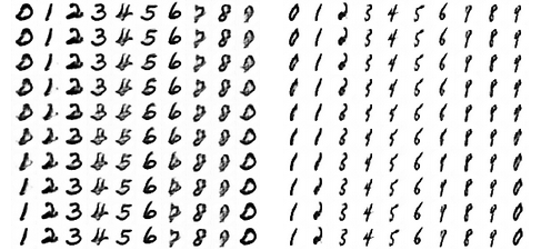

You can start to get a feeling of what is going on: style features like stroke width and curvature seem to be encoded in the latent representation. In other words, each grid seems to use a different style of handwriting. You can also see on the animations on Figure 10 that transitions between digits are very smooth, an indication that the latent space yields a continuous space of real-looking images.
Now I can also do what I call a style sweep: pick two random values of z and interpolate between the two corresponding styles, for each class. See Figure 11.

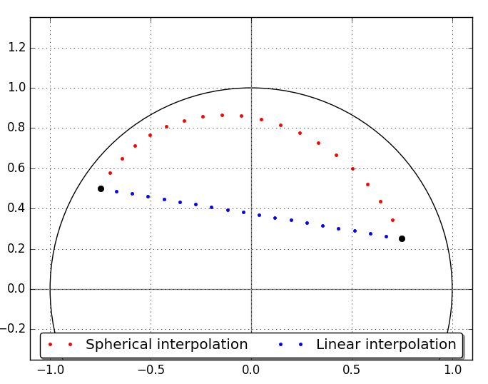
Now you might wonder how to do the interpolations in practice. Intuitively I would use a linear combination of my z vectors to perform interpolation in latent space. However intuition rarely works in a high-dimensional space. Tom White [7] points out that linear interpolation (taking the shortest path between points) leads to intermediate points that have very improbable norm and are therefore unlikely to be visited during training. That means the model may not perform well on these points. This led White to advocate the use of spherical interpolation: interpolating between two points as if walking on the surface of a high-dimensional sphere. See Figure 12 for an illustration of the difference between linear and spherical interpolation in 2D space. Spherical interpolation has become the standard way of performing interpolation in GANs. I used spherical interpolation for all examples in this post.
GAN Auto-Encoder
I can keep sampling random z vectors until I find a style that I like. But is there a more direct approach? What if I have an image of a digit in my dataset that I really like and I would like to generate all other digits using the same style?
One limitation in the standard formulation of a GAN is that there is no mapping from feature space to latent space. In other words, given a sample, there is no direct way to find the corresponding z vector. Several papers were published to address this issue, most notably [8] and [9]. Without getting into the details of the proposed solutions, they all modify the original GAN framework and provide no guarantee that the model will converge to the same solution. Feeling uneasy about this I decided to implement my own solution: I wanted to separately train an encoder, that is to say a network that outputs a z vector when given an image as input. To verify that the z vector is correct I feed it to G and then check whether the generated image is similar to the input image.
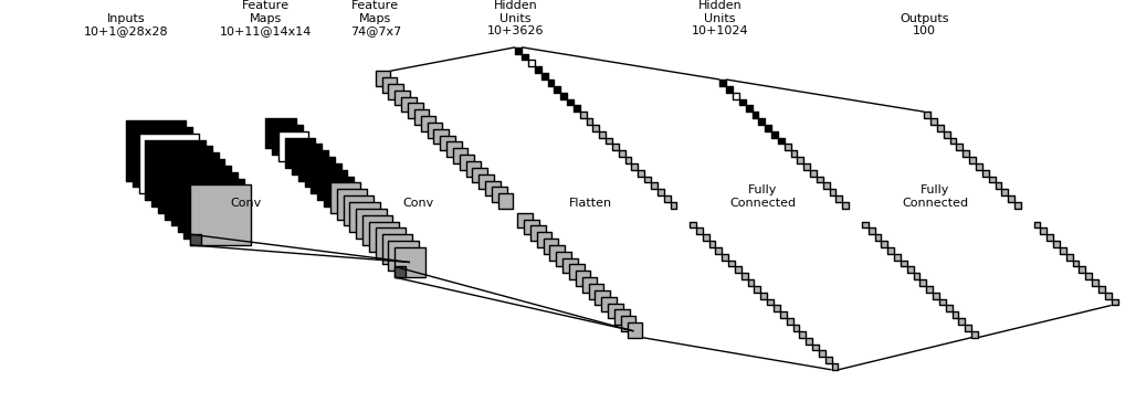
One question that arises is: how do I design a network that can extract features from my images that are useful enough to produce a good z vector? Well, I already have such a network: D! I just changed the number of output neurons in the last layer of D to 100 (the length of z), plugged the output of my modified D (let’s call it E) into G and used the L2 distance between the output of G and the input image as a loss. I have essentially reversed the order of things in my GAN and created a GAN Auto-encoder. This is utterly simple but works well enough in practice. See Figure 13 for an illustration of the encoder topology and Figure 14 for an illustration of the new set-up.
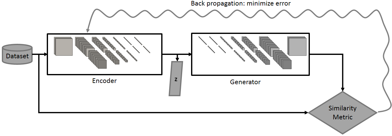
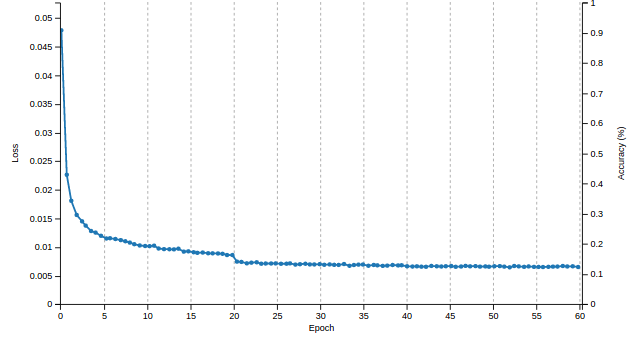
Importantly, in order to train E it is critical to initialize its weights from the weights of a trained D. In deep learning jargon, this is known as transfer learning. When I train this model in DIGITS, the learning curve is incredibly smooth, as you can see in Figure 15. I could use a more subtle similarity metric (L2 is a little bit gross here) but I found it that this simple scheme works well enough in practice.
Targeted Sampling
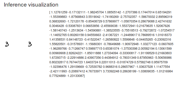
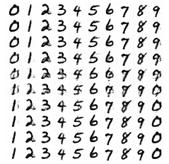
Armed with my encoder I can take an image from my dataset and find the corresponding z vector (Figure 16). Note how the reconstructed number resembles the input image.
Now It’s Your Turn!
After reading this post, you should have the information you need to get started with Generative Adversarial Networks. Download the source code now and experiment with these ideas on your own dataset. Please let us know how you are doing by commenting on this post!
Stay tuned for the second part of this post where I will show you how to use Generative Adversarial Networks to generate images of celebrity faces.
Join NVIDIA for a GAN Demo at ICLR
Visit the NVIDIA booth at ICLR Apr 24-26 in Toulon, France to see a demo based on my code of a DCGAN network trained on the CelebA celebrity faces dataset. As you’ll see in Part 2 of this series, this demo illustrates how DIGITS together with TensorFlow can be used to generate complex deep neural network architectures. Follow us at @NVIDIAAI on Twitter for updates on our ground breaking research published at ICLR.
Learn More at GTC 2017
The GPU Technology Conference, May 8-11 in San Jose, is the largest and most important event of the year for AI and GPU developers. Use the code CMDLIPF to receive 20% off registration, and remember to check out my talk, S7695 – Photo Editing with Generative Adversarial Networks. I’ll also be instructing a Deep Learning Institute hands on lab at GTC: L7133 – Photo Editing with Generative Adversarial Networks in TensorFlow and DIGITS.
Acknowledgements
I would like to thank Taehoon Kim (Github @carpedm20) for his DCGAN implementation on [6]. I would like to thank Mark Harris for his insightful comments and suggestions.
References
[1] Yann LeCun (2016). https://www.quora.com/What-are-some-recent-and-potentially-upcoming-breakthroughs-in-deep-learning
[2] Ian J. Goodfellow, Jean Pouget-Abadie, Mehdi Mirza, Bing Xu, David Warde-Farley, Sherjil Ozair, Aaron Courville, Yoshua Bengio (2014). Generative Adversarial Networks. arXiv:1406.2661
[3] Ian J. Goodfellow (2016). NIPS 2016 tutorial: Generative Adversarial Networks. arXiv:1701.00160
[4] THE MNIST DATABASE of handwritten digits. http://yann.lecun.com/exdb/mnist/
[5] Alec Radford, Luke Metz, Soumith Chintala (2015). Unsupervised Representation Learning with Deep Convolutional Generative Adversarial Networks. arXiv:1511.06434
[6] DCGAN-tensorflow. https://github.com/carpedm20/DCGAN-tensorflow
[7] Tom White (2016). Sampling Generative Networks. arXiv:1609.04468
[8] Anders Boesen Lindbo Larsen, Søren Kaae Sønderby, Hugo Larochelle, Ole Winther (2015). Autoencoding beyond pixels using a learned similarity metric. arXiv:1512.09300
[9] Vincent Dumoulin, Ishmael Belghazi, Ben Poole, Olivier Mastropietro, Alex Lamb, Martin Arjovsky, Aaron Courville (2016). Adversarially Learned Inference. arXiv:1606.00704
