Decades of computer science history have been devoted to devising solutions for efficient storage and retrieval of information. Hash maps (or hash tables) are a popular data structure for information storage given their amortized, constant-time guarantees for the insertion and retrieval of elements.
However, despite their prevalence, hash maps are seldom discussed in the context of GPU-accelerated computing. While GPUs are well known for their massive number of threads and computational power, their exceptionally high memory bandwidth enables acceleration of many data structures such as hash maps.
This post walks through the fundamentals of hash maps and how their memory access patterns make them well suited for GPU acceleration. We will introduce cuCollections, a new open-source CUDA C++ library for concurrent data structures, including hash maps.
Finally, if you are interested in using GPU-accelerated hash maps in your applications, we provide an example implementation of a multicolumn relational join algorithm. RAPIDS cuDF has integrated GPU hash maps, which helped to achieve incredible speedups for data science workloads. To learn more, see rapidsai/cudf on GitHub and Accelerating TF-IDF for Natural Language Processing with Dask and RAPIDS.
You can also leverage cuCollections for many use cases outside of tabular data processing, such as recommender systems, stream compaction, graph algorithms, genomics, and sparse linear algebra operations. See Pinterest Boosts Home Feed Engagement 16% With Switch to GPU Acceleration of Recommenders to learn more.
Hash map basics
Hash maps are associative containers, meaning they store key–value pairs where a key is mapped to an associated value, enabling the retrieval of values by looking up their keys. For example, you could use a hash map to implement a phone book by using an individual’s name as the key and their phone number as the associated value.
Hash maps are different from other associative containers in that operations, such as insertion or retrieval, have a constant cost on average. std::map in the C++ Standard Template Library is not a hash table, but is typically implemented as a binary search tree. std::unordered_map is more akin to the kind of hash tables relevant to this discussion. For the purposes of this post, there is no difference between a hash table and a hash map. Both terms will be used interchangeably throughout.
Single-value compared to multivalue
An important distinction when discussing hash tables is whether or not duplicate keys are allowed. Single-value hash tables or hash maps require keys to be unique (for example, std::unordered_map), whereas multivalue hash tables or hash multimaps allow duplicate keys (for example, std::unordered_multimap).
Using the phone book analogy, the latter refers to the case where a single individual can have more than one phone number. For example, the phone book could have (k=Alice, v=408-555-0148) and a duplicate key with another value (k=Alice, v=408-555-3847).
Storage and retrieval
Conceptually, a hash map consists of an array of buckets, where each bucket may hold one or more key-value pairs. To insert a new pair into the map, a hash function is applied to the key to yield a hash value. This hash value is then used to select one of the buckets. If the bucket is available, then the pair is stored within that bucket.
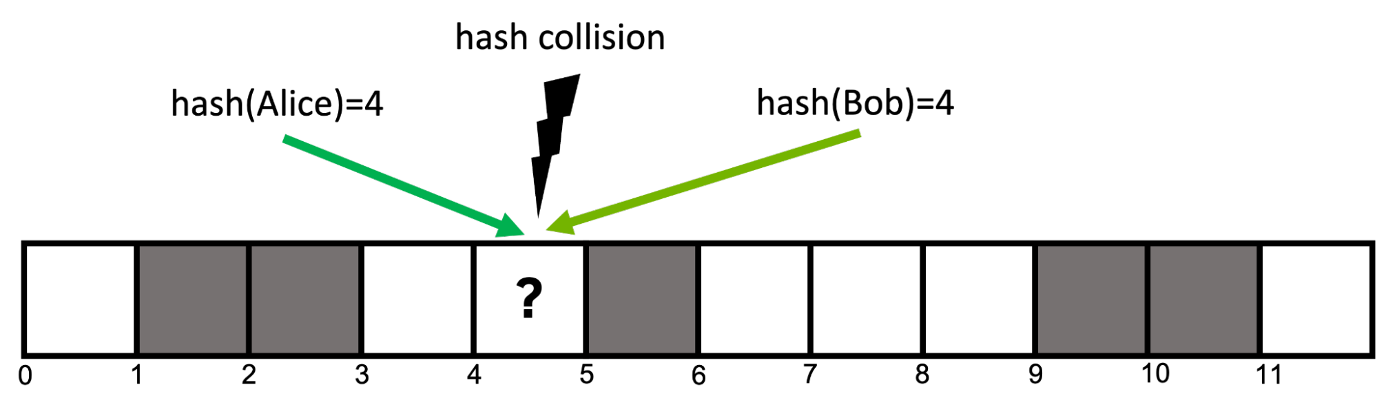
For example, to insert the pair (Alice, 408-555-0148), you hash the key, hash(Alice)=4, to get its hash value and select the bucket at position four to store the pair. Later, to retrieve the value associated with Alice, you can use the same hash function, hash(Alice), to again select the bucket at position four and retrieve the previously stored value.
Hash collisions
If the number of buckets in the table is equal to the number of possible keys, a one-to-one relation between hash buckets and keys can be employed, where each key maps to exactly one bucket in the table.
However, this is impractical in most cases because either the number of potential keys is not known in advance or the storage required to reserve a bucket for each key would exceed the available memory capacity. Imagine if your phone book had to reserve an entry for every possible name in the universe!
As a result, hash functions are usually imperfect and can result in hash collisions, where two distinct keys map to identical hash values (Figure 1). Good hash functions seek to minimize the likelihood of collisions, but they are unavoidable in most cases.
Open addressing
There are numerous strategies for resolving hash collisions that can be found in literature, but this post focuses on a strategy called open addressing with linear probing.
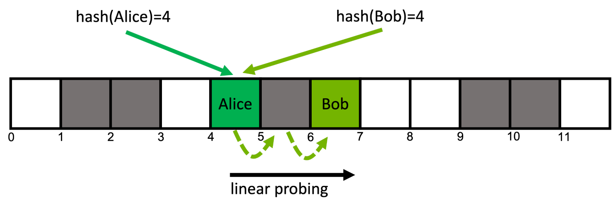
An open addressing hash table uses a contiguous array of buckets in memory. With linear probing, if an already-occupied bucket is encountered at position i, you move to the next adjacent position i+1. If this bucket is also occupied, you move to i+2, and so on. When you reach the last bucket, you wrap around back to the beginning. This so-called probing scheme is deterministic for each key (Figure 2).
This approach is cache efficient because it accesses consecutive locations in memory. It can suffer performance degradation if the load factor (ratio of filled to total buckets) is high, as it leads to additional memory reads.
Retrieving the key Bob from the map works in the same fashion: follow the key’s probing sequence starting at position hash(Bob)=4 until you find the desired bucket at position six. If at any point in a given key’s probing sequence you encounter an empty bucket, you know that the queried key is not present in the map.
Random memory access
Well-designed hash functions minimize the number of collisions by maximizing the likelihood that hashing any two keys will result in distinct hash values. This means for any given two keys, their corresponding buckets are likely in disparate memory locations.
As such, the memory access pattern of most hash table operations is effectively random. To comprehend the performance of hash tables, it is important to understand the performance of random memory access.
Table 1 compares the theoretical peak bandwidth with the achieved bandwidth for random 64-bit reads, as measured by the GUPS benchmark, on modern CPUs and GPUs.
| Chip (memory) | Theoretical peak bandwidth (GB/s) | Measured random 64-bit read bandwidth (GB/s) |
| Intel Xeon Platinum 8360Y (DDR4-3200, 8 channels) | 204 | 15 |
| NVIDIA A100-80GB-SXM (HBM2e) | 2039 | 141 |
| NVIDIA H100-80GB-SXM (HBM3) | 3352 | 256 |
If you are interested in running the GUPS GPU benchmark on your system, see the NVIDIA developer blog code samples GitHub repository. You can access the CPU code in the ParRes/Kernels GitHub repository.
As you can see, random memory access is approximately 10x slower than the theoretical peak bandwidth. This is because memory subsystems are optimized for sequential accesses. More importantly, the random access throughput of NVIDIA GPUs is an order of magnitude more than that of modern CPUs. These results indicate that the best-performing CPU hash table is likely to be an order of magnitude slower than the best-performing GPU hash table.
GPU hash map implementation
Random memory accesses are inevitable in hash table implementations, and GPUs excel at random access compared to CPUs. This is promising as it hints that GPUs should excel at hash table operations. To test this theory, this section discusses the implementation and optimization of a GPU hash table, comparing the performance to CPU implementations.
The goal is not to develop a drop-in replacement for standard C++ containers such as std::unordered_map, but to focus on implementing a hash table that is suited to the kinds of massively parallel, high-throughput problems that arise in GPU-accelerated applications.
This example uses the following simplifying assumptions:
- the capacity of the table is fixed—additional key-value pairs cannot be added beyond the initial capacity
- one of the possible key values needs to be set aside as a sentinel value to indicate an empty bucket
- the sum of the sizes of the key and value types must be less than or equal to eight bytes
- key-value pairs cannot be deleted once inserted
Note that these are not fundamental limitations and can be overcome with more advanced implementations that are provided in the cuCollections library.
To start, the example hash table uses open addressing and consists of an array of buckets. Each bucket can hold a single key-value pair and is initialized with the key/value sentinels to denote that it is currently empty. For collision resolution, linear probing is used.
A GPU-accelerated hash table needs to support concurrent updates from many threads and it is necessary to take steps to avoid data races—for example, if two threads attempt to insert at the same location. To avoid expensive locking, the example hash table uses atomic operations through cuda::std::atomic from libcu++ where each bucket is defined as cuda::std::atomic<pair<key, value>>.
To insert a new key, the implementation computes the first bucket from its hash value and performs an atomic compare-and-swap operation with the expectation that the key in the bucket is equal to empty_sentinel. If so, the slot was empty and the insert succeeds. Otherwise, it advances to the next bucket until it eventually finds an empty bucket.
The code below shows a simplified version of the hash table insert function.
__device__ bool insert(Key k, Value v) {
// get initial probing position from the hash value of the key
auto i = hash(k) % capacity;
while (true) {
  // load the content of the bucket at the current probe position
  auto [old_k, old_v] = buckets[i].load(memory_order_relaxed);
  // if the bucket is empty we can attempt to insert the pair
  if (old_k == empty_sentinel) {
    // try to atomically replace the current content of the bucket with the input pair
    bool success = buckets[i].compare_exchange_strong(
                    {old_k, old_v}, {k,v}, memory_order_relaxed);
    if (success) {
      // store was successful
      return true;
    }
  } else if (old_k == k) {
    // input key is already present in the map
    return false;
  }
  // if the bucket was already occupied move to the next (linear) probing position
  // using the modulo operator to wrap back around to the beginning if we
  // go beyond the capacity
  i = ++i % capacity;
}
}
Looking up the associated value of a specific key in the map works in a similar fashion. Inspect each position along the key’s probing sequence until either a bucket that contains the desired key, or an empty bucket is found, indicating that the key cannot be resident within the table.
Cooperative groups
Assigning one worker thread to each input element may at first seem like a reasonable ratio. However, consider the following:
- There is no relation between neighboring keys in the input and their associated probing location in memory. This implies that every thread in a warp is likely accessing a completely different region of the hash map. In the worst-case scenario, each warp needs to load from 32 distinct locations in global memory per probing step. (Recall the random memory access.)
- With linear probing, each thread may access multiple adjacent buckets starting at its initial probing position. This local access pattern would allow for prefetching multiple probing positions with a single coalesced load, which unfortunately cannot be achieved with a single thread.
Can we do better? Yes. The CUDA cooperative groups model enables reconfiguring the granularity of work-assignment with ease. Instead of using a single CUDA thread per input element, an element is assigned to a group of consecutive threads inside the same warp.
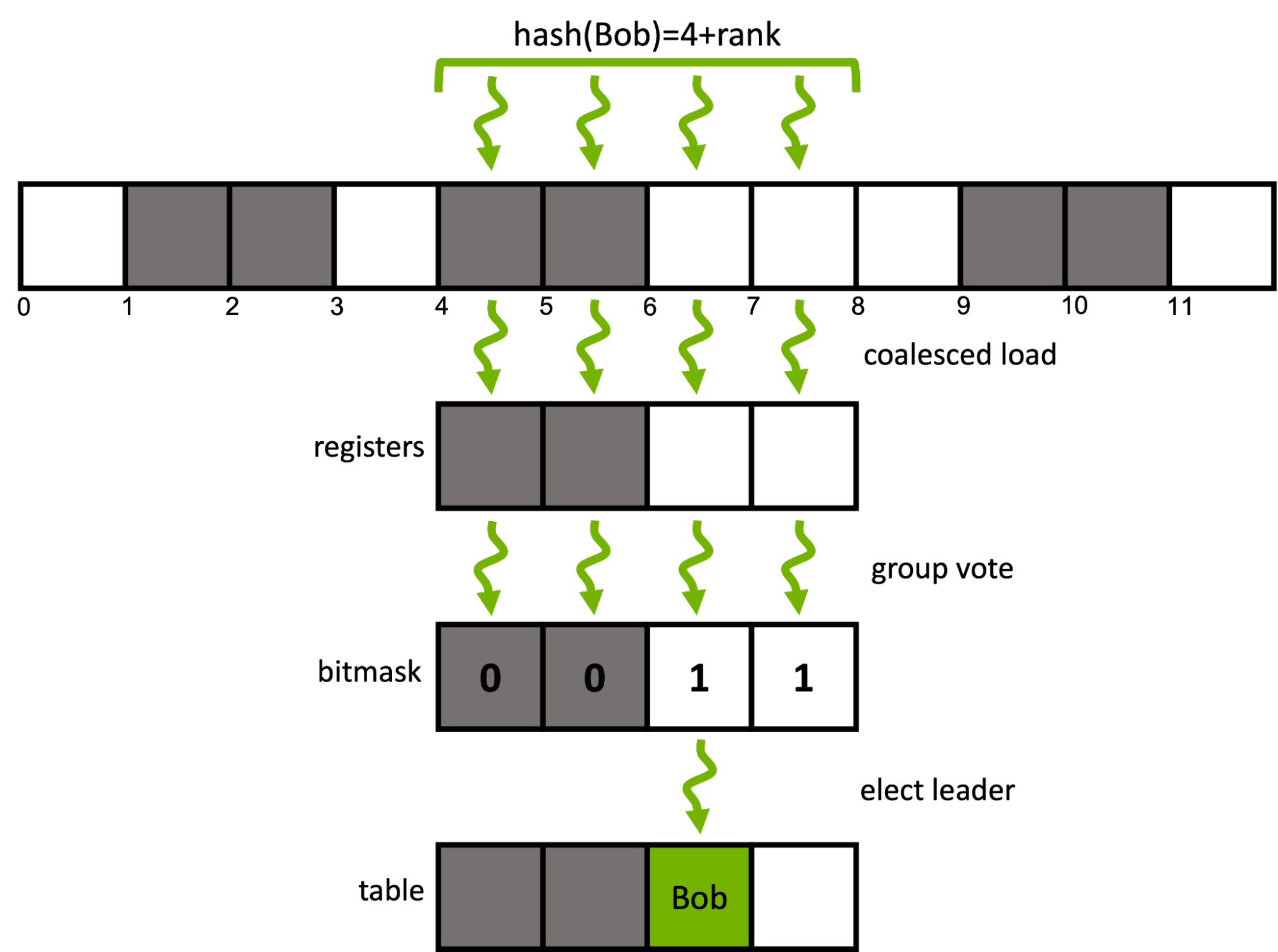
For a given input key, instead of traversing its associated probing sequence sequentially, a window of multiple adjacent buckets is prefetched with a single coalesced load. The group then cooperatively determines a candidate bucket inside the window using efficient ballot and shuffle intrinsics.
The following code extends the previously introduced insert function to use four consecutive threads within a warp to cooperatively insert a single key. cg::thread_block_tile<4> represents the four threads in the subwarp.
enum class probing_state { SUCCESS, DUPLICATE, CONTINUE };


__device__ bool insert(cg::thread_block_tile<4> group, Key k, Value v) {
// get initial probing position from the hash value of the key
auto i = (hash(k) + group.thread_rank()) % capacity;
auto state = probing_state::CONTINUE;
while (true) {
  // load the contents of the bucket at the current probe position of each rank in a coalesced manner
  auto [old_k, old_v] = buckets[i].load(memory_order_relaxed);
  // input key is already present in the map
  if(group.any(old_k == k)) return false;
  // each rank checks if its current bucket is empty, i.e., a candidate bucket for insertion
  auto const empty_mask = group.ballot(old_k == empty_sentinel);
  // it there is an empty buckets in the group's current probing window
  if(empty_mask) {
    // elect a candidate rank (here: thread with lowest rank in mask)
    auto const candidate = __ffs(empty_mask) - 1;
    if(group.thread_rank() == candidate) {
      // attempt atomically swapping the input pair into the bucket
      bool const success = buckets[i].compare_exchange_strong(
                      {old_k, old_v}, {k, v}, memory_order_relaxed);
      if (success) {
        // insertion went successful
        state = probing_state::SUCCESS;
      } else if (old_k == k) {
        // else, re-check if a duplicate key has been inserted at the current probing position
        state = probing_state::DUPLICATE;
      }
    }
    // broadcast the insertion result from the candidate rank to all other ranks
    auto const candidate_state = group.shfl(state, candidate);
    if(candidate_state == probing_state::SUCCESS) return true;
    if(candidate_state == probing_state::DUPLICATE) return false;
  } else {
    // else, move to the next (linear) probing window
    i = (i + group.size()) % capacity;
  }
}
}
The preceding code samples for the hash table insert function are a simplified version of the actual implementation of the cuCollections cuco::static_map.
Figure 4 shows the performance of the noncooperative and cooperative probing approaches with no materialization for different group sizes and table occupancies measured on an NVIDIA A100 80 GB GPU.
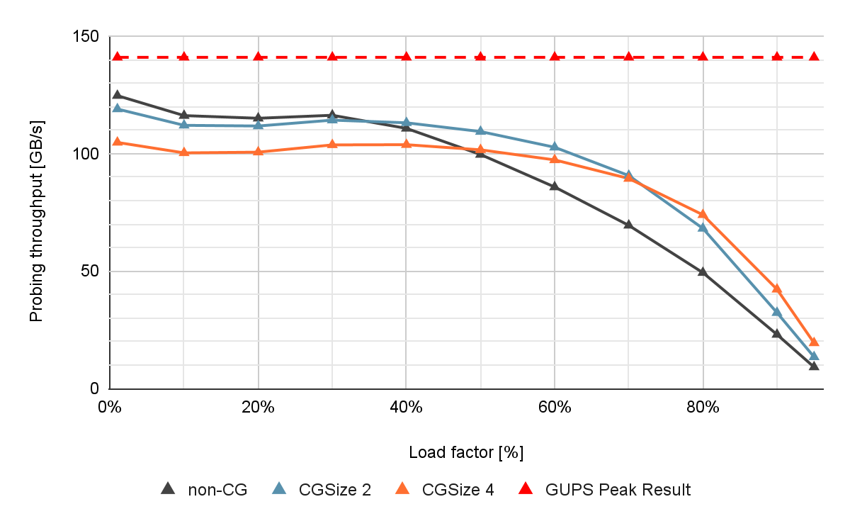
If the load factor is low, the noncooperative (non-CG) shows close to optimal performance. However, if the load factor increases, the throughput decreases drastically due to an increased number of collisions and longer probing sequences. This is problematic because a higher table load factor corresponds to better memory utilization.
Cooperative probing improves the performance for such high load factor scenarios. With a group size of four, you can observe up to 13% higher insert throughput, and 40% higher find throughput compared to the noncooperative approach when the load factor is high.
Long probing sequences also occur in multivalue scenarios with high key multiplicities, since identical keys traverse the same sequence of buckets. Cooperative probing also helps speed up these scenarios.
For more information about group-cooperative hash table probing, see Parallel Hashing on Multi-GPU Nodes and WarpCore: A Library for Fast Hash Tables on GPUs.
Existing CPU and GPU hash maps comparison
A variety of C++ hash map implementations have been proposed over the years. Among the most popular are the libstdc++/libc++ std::unordered_map and the Abseil absl::flat_hash_map. These are sequential implementations and using them from multiple threads requires additional synchronization.
The tbb::concurrent_hash_map from TBB and folly::AtomicHashMap from Folly are examples of concurrent multithreaded CPU data structures. One of the few implementations usable from GPUs is kokkos::UnorderedMap from the Kokkos library.
Compare the performance of the map implementations provided above against the cuCollection cuco::static_map. The benchmark setup is as follows.
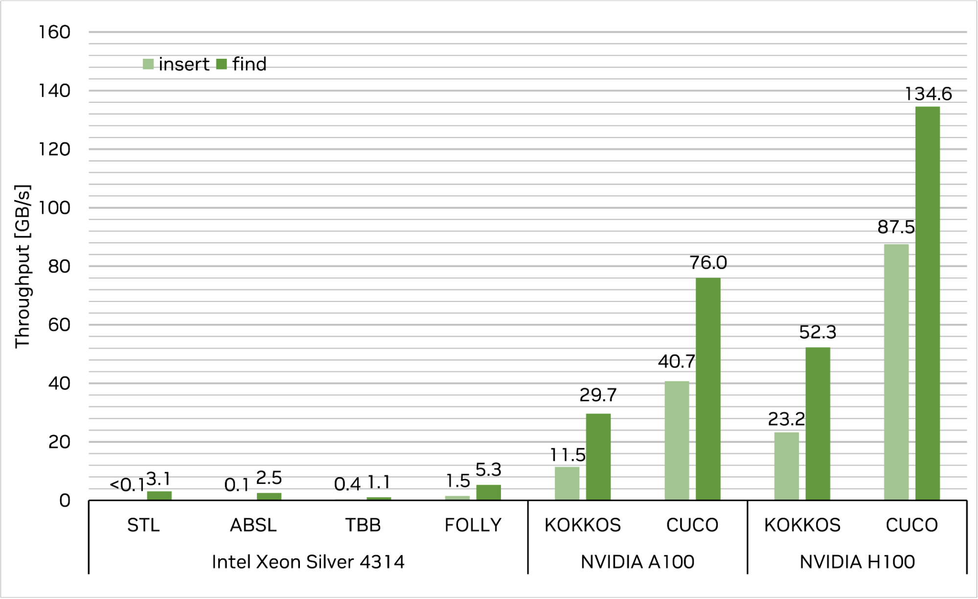
First, insert 227 (1 GB) unique 4-byte key/4-byte value pairs into each map and subsequently query the same set of keys to retrieve their associated values. The target table load factor for each run is 50%. Performance is measured in memory throughput (GB per second; higher is better).
The results are shown in Figure 5. The cuco::static_map achieves an insert throughput of 87.5 GB/s, and a find throughput of 134.6 GB/s on a single NVIDIA H100-80GB-SXM, which translates to more than order-of-magnitude speedup over the fastest CPU single-threaded and multi-threaded implementations. Additionally, cuCollections outperforms the other GPU implementation in this test, kokkos::UnorderedMap, by a factor of 3.8x for insert, and 2.6x for find, respectively.
Note that in this benchmark setup, the I/O vectors for each operation are resident in CPU memory for CPU-sided implementations, and in GPU memory for the GPU-sided implementations. If the data vectors need to be resident in CPU memory for the GPU hash maps, this would require the input data to be moved to the GPU first, and the result to be moved back to the CPU memory afterwards.
This can be achieved either through explicit (asynchronous batch) copying, or automatic page migration using CUDA’s concept of unified memory. As the results show, the achieved throughput of our implementation is always well above the practically available bandwidth of PCIe Gen4, and even PCIe Gen5 on H100. This implies that this approach is able to fully saturate the link between the CPU and the GPU.
In other words, cuCollections enables you to build and query hash tables at the speed of your system’s PCIe bandwidth even when the data is not located in GPU memory. Moreover, the NVIDIA Grace Hopper Superchip can provide additional speedup, thanks to the fast NVLink-C2C interconnect between CPU and GPU, unleashing the full throughput of the hash table. In contrast, CPU hash maps often achieve much lower throughput compared to PCIe.
Example of multicolumn relational join
This section features a real-world example of how a GPU hash table can be used to implement a complex algorithm.
cuDF is a GPU-accelerated library for data analytics. It provides primitives for data manipulations like loading, joining, and aggregating. By leveraging the cuCollections hash tables, it uses a hash join algorithm to perform join operations.
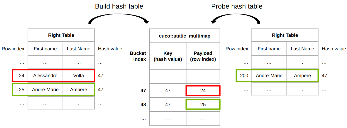
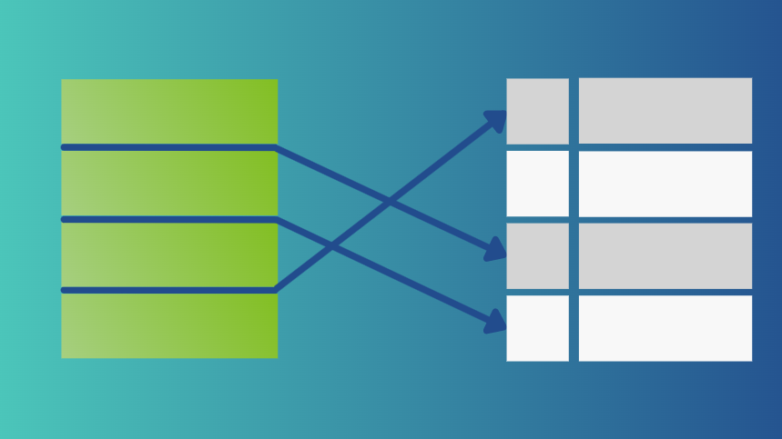
Figure 6 shows how cuDF join implementation works for an inner join. cuDF provides a built-in hash function to hash rows of arbitrary types to a hash value. Distinct rows can have the same hash value thus a row equality check is required to determine whether two rows are truly identical.
The table on the left is used to fill a cuco::static_multimap where the key is the row’s hash value and the payload is the associated row index. Row 24 is inserted at bucket 47 and row 25 is inserted at bucket 48. During the probe phase, the hash value of row 200 in the right table is 47, which is the same as the hash value (or the same key) of bucket 47 from the hash table.
To finally identify whether two rows are equal or not, the row index of {André-Marie, Ampère} from the table on the right, 200, together with the row index of {Alessandro, Volta} from the table on the left, 24, are passed to a row equality function, row_equal(200, 24).
In the end, these two rows are not identical, thus row 24 of the table on the left is not a match. Eventually, row 25 from the left table is a match of row 200 of the right table, since hash values are identical and the row equality check (row_equal(200, 25)) passes as well.
Benchmarking join operations is a complex topic given the many options for sizes, selectivity, and more. For more details, see How to Get the Most out of GPU Accelerated Database Operators and Effective, Scalable Multi-GPU Joins.
How to use GPU hash maps in your code
GPUs are a great fit for concurrent data structures like hash maps. It all starts with the high bandwidth memory architecture that is an order-of-magnitude faster than on the CPU for many small random reads and atomic updates. This directly translates into highly efficient hash table insert and probe performance on the GPU.
This post introduced a few important considerations when designing a massively parallel hash map: 1) flat memory layout for hash buckets with open addressing to resolve collisions and 2) threads cooperating on neighboring hash buckets for insertion and probing to improve performance in high load factor scenarios. You can find fast and flexible hash map implementations on GitHub as part of the cuCollections library.
If high performance data storage and retrieval is important for your application, a GPU-accelerated hash table can be your go-to data structure. Give the cuCollections library a try and experience the power of GPUs for yourself.
Register for GTC 2023 for free and join us March 20–23 to learn more about data science and how accelerated computing can transform your work.
Acknowledgements
We would like to thank Rui Lan and Lars Nyland for contributing to this post.
