Recommender systems (RecSys) have become a key component in many online services, such as e-commerce, social media, news service, or online video streaming. However with the growth in importance, the growth in scale of industry datasets, and more sophisticated models, the bar has been raised for computational resources required for recommendation systems.
To meet the computational demands for large-scale DL recommender systems, NVIDIA introduced Merlin – a Framework for Deep Recommender Systems. Now NVIDIA teams have won two consecutive RecSys competitions in a row: the ACM RecSys Challenge 2020, and more recently the WSDM WebTour 21 Challenge organized by Booking.com. The Booking.com challenge focused on predicting the last city destination for a traveler’s trip given their previous booking history within the trip. NVIDIA’s interdisciplinary team included colleagues from NVIDIA’s KGMON (Kaggle Grandmasters), NVIDIA’s RAPIDS (Data Science), and NVIDIA’s Merlin (Recommender Systems) who collaborated on the winning solution.
This post is the third of a three-part series that gives an overview of the NVIDIA team’s first-place solution for the booking.com challenge focused on predicting the last city destination for a traveler trip given their previous booking history within the trip. The first post gives an overview of recommender system concepts. The second post discusses deep learning for recommender systems. This post discusses the winning solution, the steps involved, and also what made a difference in the outcome. Specifically, this blog post explains the booking.com RecSys challenge competition goals, exploratory data analysis, feature preprocessing and extraction, the algorithms used, model training, and validation.
The Booking.com Challenge Problem Overview
Many of the booking.com users go on trips which include more than one destination and booking.com recommends a next destination. For instance, if a user was making hotel reservations for Amsterdam, Rotterdam, and Copenhagen then booking.com would immediately suggest popular cities for extending their trip such as Stockholm, Oslo, or Berlin.

Figure 1: Booking.com suggests popular options for extending a user’s trip as they make their booking.
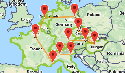
In this booking.com example for a trip to Italy, the sequence of cities shown in the blue route is more likely than the red route. Similarly, if the sequence of cities so far is Venice, Florence, Rome, then the next destination is more likely to be Palermo than Milan.

Figure 2: The sequence of cities shown in the blue route is more likely than the red route.
The goal of this challenge was to use a dataset based on millions of booking.com real anonymized hotel reservations to come up with a strategy for making the best recommendation for their last destination in real-time. Specifically, the goal was to predict (and recommend) the final city (city_id) of each trip (utrip_id). The quality of the predictions was evaluated based on the top four recommended cities for each trip by using Top-4 Accuracy metric (4 representing the four suggestion slots on the Booking.com website). When the true city is one of the top 4 suggestions, it was considered correct.
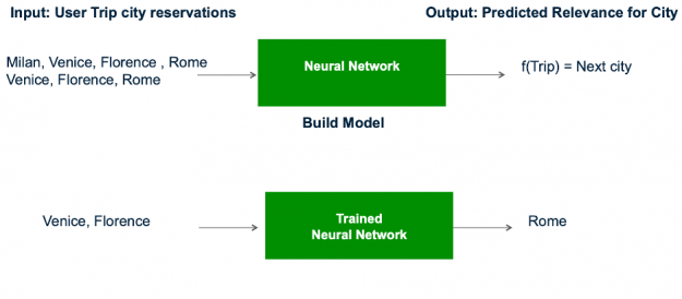
Figure 3: The goal was to predict the final destination of each trip given a dataset of real hotel reservations.
More than 800 participants signed up for the contest grouped in 40 competing teams. NVIDIA’s interdisciplinary team was represented by Benedikt Schifferer, Chris Deotte, Jean-François Puget, Gabriel de Souza, Pereira Moreira, Gilberto Titericz, Jiwei Liu, and Ronay Ak. The winning NVIDIA team achieved Accuracy @ 4 of 0.5939, using a blend of Transformers, GRUs, and feed-forward multi-layer perceptron.
The Competition Process
RecSys or Kaggle competitions work by asking users or teams to provide solutions to well-defined problems. Competitors download the training and test files, train models on the labeled training file, generate predictions on the test file, and then upload a prediction file as a submission. After you submit your solution, you get a ranking. At the end of the competition, the top scores are announced as winners.
A general data science process and competition tip are to set up a fast experimentation pipeline on GPUs, where you train, improve the features and model, and then validate repeatedly. The NVIDIA team used a fast experimentation pipeline on GPUs consisting of preprocessing and feature engineering with RAPIDS cuDF, a library for GPU-accelerated dataframe transformations, combined with TensorFlow and PyTorch for deep learning. The RAPIDS suite of open-source software libraries, built on CUDA, gives you the ability to execute end-to-end data science and analytics pipelines entirely on GPUs, while still using familiar interfaces like Pandas and Scikit-Learn APIs.
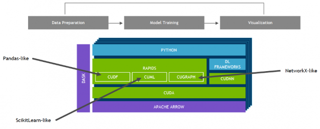
Figure 4: End-to-End Data science pipeline with GPUs and RAPIDS.
Exploratory Data Analysis
Exploratory data analysis (EDA) is performed before, during, and after feature engineering to understand the dataset better. EDA uses data visualization, statistics, and queries to find important variables, interesting relations among the variables, anomalies, patterns, and insights.
The training dataset consists of a csv file with 1.5 million anonymized hotel reservations, based on real data, with the following features:
- User_id – User ID
- Check-in – Reservation check-in date
- Checkout – Reservation check-out date
- Affiliate_id – An anonymized ID of affiliate channels where the booker came from (e.g. direct, some third-party referrals, paid search engine, etc.)
- Device_class – desktop/mobile
- Booker_country – Country from which the reservation was made (anonymized)
- Hotel_country – Country of the hotel (anonymized)
- City_id – city_id of the hotel’s city (anonymized)
- Utrip_id – Unique identification of user’s trip (a group of multi-destination bookings within the same trip)
Each reservation is a part of a customer’s trip (identified by utrip_id) which includes at least 4 consecutive reservations. The evaluation dataset is constructed similarly, however the city_id of the final reservation of each trip is concealed and requires a prediction.
The sequence of user trip reservations can be obtained by sorting on the user_id and check-in date. Below, we read in the train and test data from the csv files using cuDF, sort on the userid, check-in date to obtain the sequence of trip reservations for a user. A count on the sorted dataset reveals 269k trips.
train = cudf.read_csv('../00_Data/booking_train_set.csv').sort_values(by=['user_id','checkin'])
test = cudf.read_csv('../00_Data/booking_test_set.csv').sort_values(by=['user_id','checkin'])


print(train.shape, test.shape)
train.head()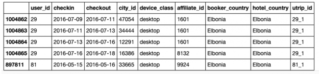
Visualizing the data can help with preprocessing and feature selection by revealing trends in the data. Histograms or bar charts help visualize the distribution of a feature. For example, the count vs. the city id frequency chart below shows that the distribution of the city reservation frequency was long-tailed as one would expect – some cities are much more popular for tourism and business than others. To help the models to focus less on very unpopular cities (city reservation frequency < 9 in this case), their city id was assigned to a single value for training to ensure that those cities were never ranked high during inference. This approach reduced the cardinality of the cities from more than 44,000 to about 11,000 cities.
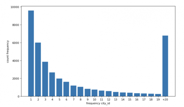
Figure 5: Distribution of frequency of city_id in train and test dataset. Around 10,000 city ids appeared only once in the dataset.
Feature Pre-Processing, Selection, and Generation
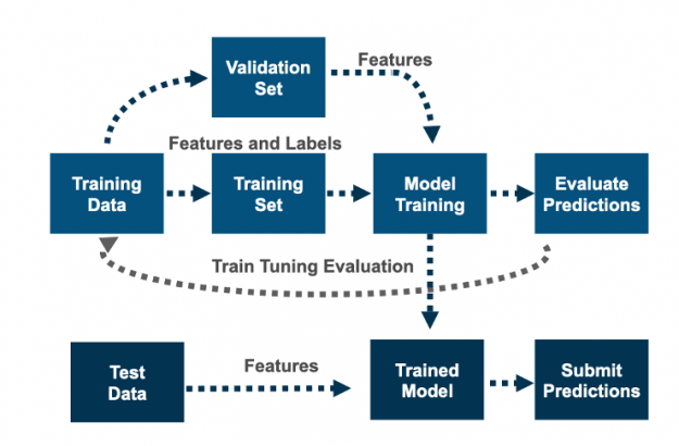
Feature engineering and feature selection is an iterative process that starts with engineering new features, then training a model, and then evaluating the model predictions against the target labels. The goal is to determine which features improve the model’s prediction accuracy. You repeat this process, along with hyperparameter tuning, until you are satisfied with the model’s accuracy.
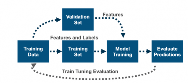
Figure 6: Machine learning is an iterative process involving feature engineering, training, testing, and tuning.
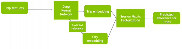
Framing this problem under the recommender systems taxonomy, the cities are the items we want to recommend for a trip. The trip is analogous to a session in the session-based recommendation task (see part 2 of this series), which is generally a sequence of user interactions – city hotel reservations in this case.
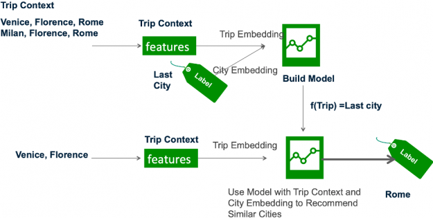
Figure 7: The recommender model learns the trip and city embeddings based on the trip features and last city (label) which are then used by the trained model to infer similar next cities.
Feature generation creates new features using knowledge about the problem and data. Feature columns can be combined, subtracted, counted, aggregated, and transformed to create new features to describe the user session (the Trip) and the cities. The NVIDIA team created the following additional features from the original 9:
- Trip context date, time features: day-of-week, week-of-year, month, weekend, season, stay length (checkout – check-in), days since the last booking (check-in – previous checkout).
- Trip context sequence features: the first city in the trip, lagged (previous 5) cities and countries from the trip.
- Trip context statistics: trip length (number of reservations), trip duration (days), reservation order (in ascending and descending orders).
- Past user trip statistics: number of user’s past reservations, number of user’s past trips, number of user’s past visited cities, number of user’s past visited countries.
- Geographic seasonal city popularity: features based on the conditional probabilities of a city c from a country co, being visited at a month m or at a week-of-year w, as follows: P(c | m), P(c | m, co), P(c | w), P(c | w, co).
The dataset with 1.5M bookings is relatively small in comparison to other recommendation datasets. Techniques were explored to increase the training data by data augmentation and the team discovered that doubling the dataset with reversed trips improved the model’s accuracy. A trip is an ordered sequence of cities and although there are many permutations to visit a set of cities, there is a logical ordering implied by distances between cities and available transportation connections. These characteristics are commutative. For example, a trip of Boston->New York->Princeton->Philadelphia->Washington DC can be booked in reverse order, but not many people would book in a random order like Boston->Princeton->Washington DC->New York->Philadelphia.
Machine Learning Algorithms Used by the Winning Team
Ensemble methods combine multiple machine learning algorithms to obtain a better model. For the winning solution, the final submission was a simple ensemble (weighted average) of the predictions from models of three different neural architectures: Multilayer perceptron with Session-based Matrix Factorization net (MLP-SMF), Gated Recurrent Unit with MultiStage Session-based Matrix Factorization net (GRU-MS-SMF), and XLNet (Transformer) with Session-based Matrix Factorization net (XLNet-SMF). As the cardinality of the label (city) is not large, all models treated the recommendation as a multi-class classification problem, by using softmax cross-entropy loss function.
In deep learning, the last layer of a neural network used for classification can often be interpreted as a logistic regression. In this context, one can see a deep learning algorithm as multiple feature learning stages, which then pass their features into a logistic regression that classifies an input. The softmax function is a generalization of logistic regression often used to normalize the output of a neural network to a probability distribution over predicted output classes for multi-class classification.
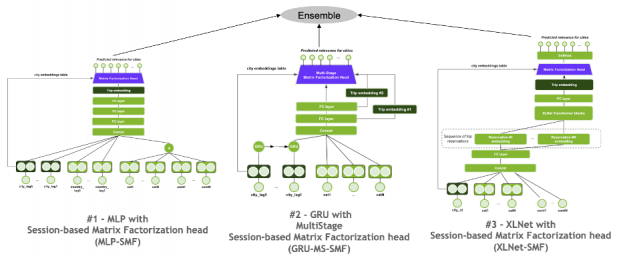
Figure 8: The final submission was an ensemble of the predictions from models of three different neural architectures.
Session-based Matrix Factorization Layer
A shared component among the three different neural architectures was a Session-based Matrix Factorization (SMF) layer, which learns a linear mapping between the item (city) embeddings and the session (trip) embeddings to generate recommendations (the scores (logits) for cities) by a dot product operation.
This design was inspired by the MF-based Collaborative Filtering (see part 1), which learns latent factors for users and items by performing a dot product of their embeddings to predict the relevance of an item for a user.
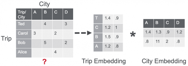
The large majority of users had only a single trip available in the dataset. So, instead of trying to model the user preference, the last layer of the network is used to represent the session (trip) embedding. Then, the dot product is computed between the session embedding s and all the set I of item embeddings i, where i is an element of I, to model items relevance probability distribution r of each item (city) being the next for that session (trip), such as r = softmax(s * I).
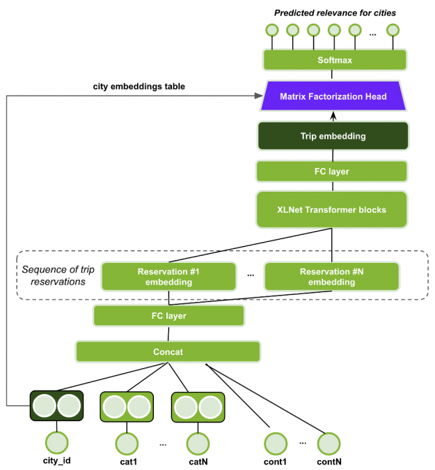
MLP with Session-based Matrix Factorization head (MLP-SMF)
The MLP with Session-based Matrix Factorization head (MLP-SMF) uses feedforward and embedding layers, as seen in Figure 11.
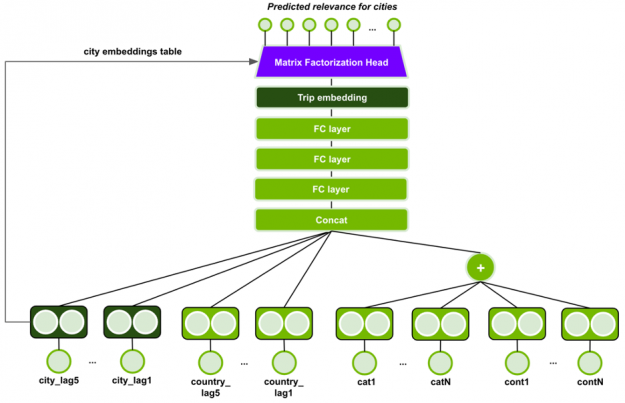
Categorical input features are fed through an embedding layer and continuous input features are individually projected via a linear layer to embeddings, followed by batch normalization and ReLU non-linear activation. All embedding dimensions are made equal. The embeddings of continuous input features and categorical input features, except the lag features, are combined via summation. The output is concatenated with the embeddings of the 5 last cities and countries (lag features).
The embedding tables for the city lags are shared, and similarly for hotel country lags. The lag embeddings are concatenated, but the model should still be able to learn the sequential patterns of cities by the order of lag features, i.e., city lag1’s embedding vector is always in the same position of the concatenated vector. The concatenated vector is fed through 3 feed-forward layers with batch normalization, PReLU activation function and dropout, to form the session (trip) embedding. It is used by the Session-based Matrix Factorization head to produce the scores for all cities.
GRU with MultiStage Session-based Matrix Factorization head (GRU-MS-SMF)
The GRU with MultiStage Session-based Matrix Factorization head uses a GRU cell for embedding the historical user actions (previous 5 visited cities), similar to GRU4Rec. (see part 2 for more information on GRUs and session based recommenders). Missing values (sequences with less than 5 length) are padded with 0s. The last GRU hidden state is concatenated with the embeddings of the other categorical input features, as shown in Figure 12.
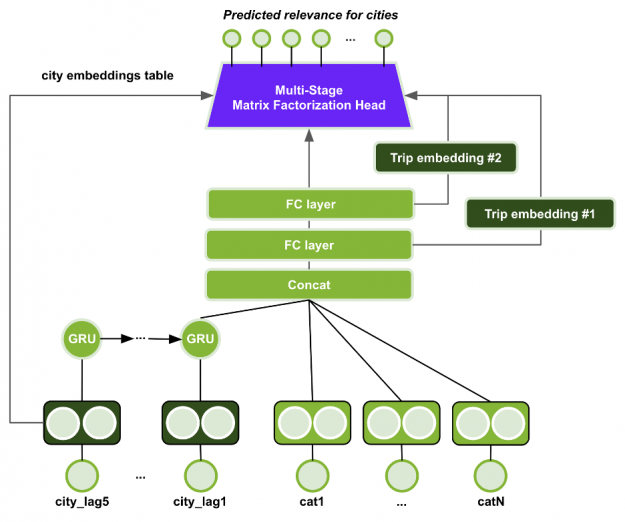
The embedding tables for the previous cities are shared. The model uses only categorical input features, including some numerical features modeled as embeddings such as trip length and reservation order. The concatenated embeddings are fed through a MultiStage Session-based Matrix Factorization head. The first stage in the MS-SMF is a softmax head over all items, which is used to select the top-50 cities for the next stage. In the second stage, the Session-based Matrix Factorization head is applied using only the top-50 cities of the first stage and two representations of the trip embeddings (the outputs of the last and second-to-last MLP layers, after the concatenation), resulting in two additional heads. The final output is a weighted sum of all three heads, with trainable weights. The multi-stage head works as a 2-stage ranking problem. The first head ranks all items and the other two heads can focus on the reranking of the top-50 items from the first stage. This approach can potentially scale to large item catalogs, i.e., in the order of millions. This dataset did not require such scalability, but this multi-stage design might be effective for deployment in production.
XLNet with Session-based Matrix Factorization head (XLNet-SMF)
The XLNet with Session-based Matrix Factorization head (XLNet-SMF) uses a Transformer architecture named XLNet, originally proposed for the permutation-based language modeling task in Natural Language Processing (NLP). In this case, the sequence of items in the session (trip) are modeled instead of the sequence of word tokens (see part 2 for more information on transformers and session based recommenders).
The XLNet training task was adapted for Masked Language Modeling (also known as Cloze task), like proposed by BERT4Rec for sequential recommendation. In that approach, for each training step, a proportion of all items are masked from the input sequence (i.e., replaced with a single trainable embedding), and then the original ids of the masked items are predicted using other items of the sequence, from both left and right sides. When a masked item is not the last one, this approach allows the usage of privileged information of the future reservations in the trip during training. Therefore, during inference, only the last item of the sequence is masked, to match the sequential recommendation task and to not leak future information of the trip.
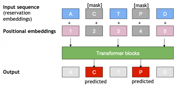
For this network, each example is a trip, represented as a sequence of its reservations. The reservation embedding is generated by concatenating the features and projecting using MLP layers. The sequence of reservation embeddings is fed to the XLNet Transformer stacked blocks, in which the output of each block is the input of the next block. The final transformer block output generates the trip embedding.
Finally, the Matrix Factorization head (dot product between the trip embedding and city embeddings) is used to produce a probability distribution over the cities for the masked items in the sequence.
Evaluating the Model
To evaluate a model’s accuracy, you test the model’s predictions, in this case the final city (city_id) of each trip, against the labeled outcome. To do this, you split the training dataset, which has labeled data, train the model on part of the data, and evaluate the predictions with the rest. For this competition, the evaluation metric was Precision@4. Precision at 4 corresponds to the proportion of top-scoring results that are relevant, in this case scoring as correct if the top-4 recommendations include the last city.
Training and Hyperparameter Tuning
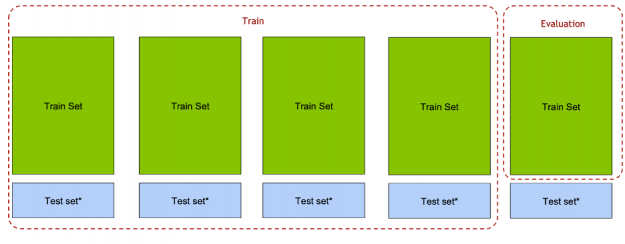
Unlike most competitions, this competition allowed only two submissions (predictions on the unlabeled test file). Because it was key to select the best features, hyperparameters and models for the final submission, it was crucial to design a good validation set. For this reason the team used k-fold cross validation, a method that maximizes the training dataset for training, tuning and evaluating a model. With cross-validation, the data is randomly split into k partitions (folds). Each fold is used one time as the validation dataset, while the rest (Out-Of-Fold – OOF) are used for training. Models are trained using the OOF training sets and evaluated with the validation sets, resulting in k model accuracy measurements.
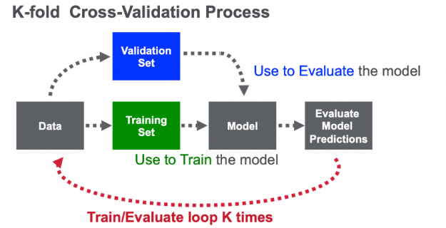
The NVIDIA team used 5-fold cross validation, using both the train data (from train.csv) and test data (test.csv), this is unusual since the test.csv data does not have the final city, but it does have a sequence of cities. For each fold, the fold train data was used for evaluation and data (both train and test) from the other folds (Out-Of-Fold – OOF) was used to train the model. The full OOF dataset was used, predicting the last city given previous ones. The Cross-Validation (CV) score was the average Precision@4 from each of the five folds.
Hyperparameter optimization tunes the model’s properties that can be set for training to find the most accurate possible model; for example the learning rate, learning rate decay, or batch size. The choice of optimal hyperparameters is between underfitting and overfitting a model—where the model predictions match how the training data behaves and is also generalized enough to make accurate predictions on unseen data. When working with neural networks, the choice of hyperparameters can make the difference between poor and superior predictive performance. To find out more about how the NVIDIA team tuned the model hyperparameters see the appendix in this whitepaper: Using Deep Learning to Win the Booking.com WSDM WebTour21 Challenge on Sequential Recommendations.
Ensembling
Ensembling is a proven approach to improve the accuracy of models, by combining their predictions and improving generalization. K-fold cross-validation and bagging techniques were used to ensemble models from the three architectures, as shown in Figure 17.
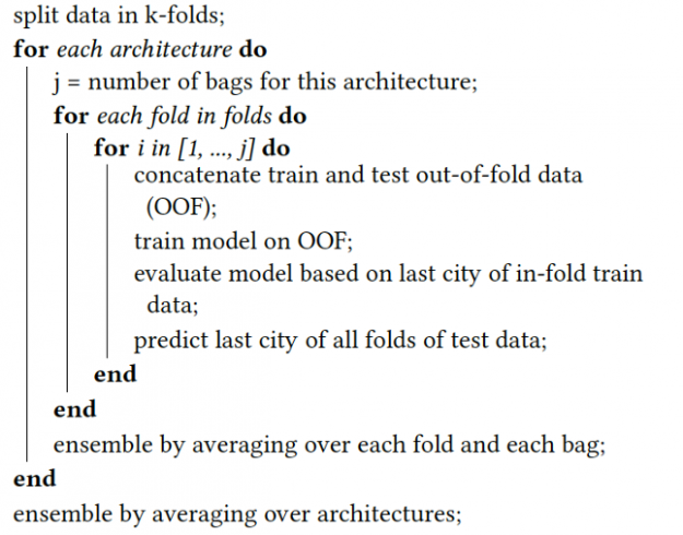
In general, the higher the diversity of the model’s predictions, the more the ensembling technique can potentially improve the final scores. In this case, the correlation of the predicted city scores between each two combinations of the three architectures was around 80%, which resulted in a representative improvement with ensembling in the final CV score.
Final Model Predictions Submission
The final step (which in this competition allowed only two submissions per team) was to submit the teams top four city predictions per each trip on the test set in a csv file named submission.csv with the following columns:
utrip_id, city_id_1, city_id_2, city_id_3, city_id_4
1000031_1, 8655, 8652, 4323, 4332
The NVIDIA team’s final leaderboard result was 0.5939 for precision@4 and scored 2.8% better than the second solution.
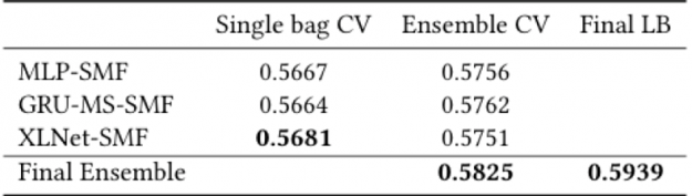
In order to clarify the contribution from each architecture and from the ensembling algorithm for the final result, the table below shows the cross-validation Precision@4 results by architecture, individual and after bagging ensembling, and the final ensemble from the three architectures combined. XLNet-SMF was the most accurate single model. The MLP-SMF architecture achieved a CV score comparable to the other two architectures that explicitly model the sequences using GRU and XLNet (Transformer). As the MLP-SMF model was lightweight, it was much faster to train than the other architectures, which sped up its experimentation cycle and improvements.
Summary
In this blog, we walked through the process of how NVIDIA’S team won the Booking.com WSDM WebTour 21 Challenge. We went over the domain problem, winning techniques in EDA, feature preprocessing, and generation, the DL models, and validation for improving predictions. The NVIDIA team designed three different deep learning architectures based on MLP, GRU, and Transformer neural building blocks. Some techniques resulted in improved performance for all models, like the Session-based Matrix Factorization head and the data augmentation with reversed trips. The diversity of the model architectures resulted in significant accuracy improvements by ensembling model predictions. We hope this post, the solution, and the links below, are useful to others interested in building recommendation systems.
Additional Resources:
- Learn more about Merlin:
- Learn How Kaggle Makes GPUs Accessible to 5 Million Data Scientists
- Competition Page: Home | Booking.com WSDM challenge
- A paper about this solution: Using Deep Learning to Win the Booking.com WSDM WebTour21 Challenge on Sequential Recommendations
- You can find the code here: https://github.com/rapidsai/deeplearning/tree/main/WSDM2021
- Learn more about NVIDIA Accelerated Data Science: GPU Accelerated Solutions for Data Science | NVIDIA
- Learn more about the other winning solutions:
- Watch GTC sessions:
- Watch Video:
