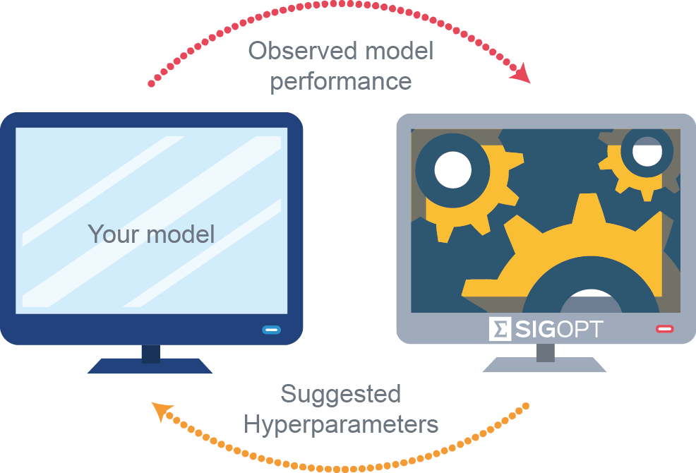
In this post we’ll show how to use SigOpt’s Bayesian optimization platform to jointly optimize competing objectives in deep learning pipelines on NVIDIA GPUs more than ten times faster than traditional approaches like random search.
Measuring how well a model performs may not come down to a single factor. Often there are multiple, sometimes competing, ways to measure model performance. For example, in algorithmic trading an effective trading strategy is one with high portfolio returns and low drawdown. In the credit card industry, an effective fraud detection system needs to accurately identify fraudulent transactions in a timely fashion (for example less than 50 ms). In the world of advertising, an optimal campaign should simultaneously lead to higher click-through rates and conversion rates.
Optimizing for multiple metrics is referred to as multicriteria or multimetric optimization. Multimetric optimization is more expensive and time-consuming than traditional single metric optimization because it requires more evaluations of the underlying system to optimize the competing metrics.

When working with neural networks and machine learning pipelines, there are dozens of free configuration parameters (hyperparameters) you need to configure before fitting a model. The choice of hyperparameters can make the difference between poor and superior predictive performance. In this post we demonstrate that traditional hyperparameter optimization techniques like grid search, random search, and manual tuning all fail to scale well in the face of neural networks and machine learning pipelines. SigOpt provides optimization-as-a-service using an ensemble of Bayesian optimization strategies accessed via a REST API, allowing practitioners to efficiently optimize their deep learning applications faster and cheaper than these standard approaches.
We explore two classification use cases, one using biological sequence data and the other using natural language processing (NLP) from a previous blog post on the AWS AI blog.
In both examples we are tuning deep neural networks exposing stochastic gradient descent (SGD) hyperparameters as well as the architecture parameters of the neural network using both MXNet and Tensorflow (code available here). We compare SigOpt and random search on the time and computational cost it takes to conduct the search as well as the quality of the models produced.
Competing Metrics in Deep Learning:
Accuracy vs. Inference Time
In deep learning, a common tradeoff is between model accuracy and speed of making a prediction. A more complex network may be able to achieve higher accuracy, but at the cost of slower inference time due to the greater computational burden associated with a larger, deeper network (See Figure 1). For example, increasing the number of filters for a particular convolutional layer, or adding more convolutional layers, will increase the number of computations needed to make an inference and thus the time required to do so. Unfortunately, it quickly becomes intractable to theoretically determine the inference time for a particular architecture. Every neural network library has a different low-level implementation, so performance must be observed empirically.
![Figure 1: An example architecture of a fully convolutional network where we expose the kernel size and number of kernels for each of the three layers as hyperparameters. The number of layers and the number of filters increase the complexity of the network, which can improve accuracy, often at the cost of increased training time. NVIDIA GPUs allow for the parallelization of computing across filters, but the computation across layers is an inherently sequential process. Image motivated by [Wang et. al. 2016].](https://developer.nvidia.com/blog/parallelforall/wp-content/uploads/2017/08/CNN-Comparison.png)
Objective Evaluation In a Multimetric Setting
Determining model performance in multimetric optimization is a difficult problem. For example, in a fraud detection model: it may be that configuration A results in a .96 F-score but takes 3 seconds to classify a given transaction, while configuration B results in a .955 F-score but takes only 20 ms for classification. Configuration A has a higher F-score than configuration B, but also takes significantly longer to classify each transaction. Each of these configurations could be optimal in a different setting, depending on the relative business tradeoffs being made. On the other hand, we don’t need to consider configuration C (.95 F-score, 200 ms), because it is strictly worse than configuration B in both metrics.
When conducting multimetric optimization, the solutions which are considered the best are those for which no other solution is strictly better. It’s hard to compare the remaining solutions, because they have strengths and weaknesses in both metrics (for example configurations A and B above). These configurations are called the efficient frontier (or Pareto frontier) and are assessed after optimization when the explicit tradeoffs can be considered.
Optimization Loop
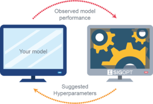 With a defined hyperparameter space, we have the following trial-and-error workflow:
- Suggest a specific model architecture and SGD parameter configuration;
- Train the model according to this configuration;
- Observe inference time and accuracy;
- Repeat steps (1) to (4) until budget exhausted;
- Return the set of “efficient” configurations.
Let’s dive in and compare Bayesian optimization via SigOpt with the common hyperparameter optimization technique of random search on two classification tasks.
Use Case 1: Sequence Data in a Biological Setting

This analysis involves diatoms, a type of algae distinguished by cell walls made of silica. The distribution of diatoms varies with climate and ecosystemic conditions, so classifying and analyzing those distributions can provide insight into past, present and future environmental conditions. Diatom classification is also applied in water quality monitoring and forensic analysis.
We use SigOpt to tune the hyperparameters of a neural network in order to accurately and quickly classify diatoms by constructing a multimetric optimization problem to simultaneously maximize accuracy and minimize inference time on a validation dataset (a dataset not seen during model training). This sequential dataset contains approximately 800 samples of length 176 and 37 diatom classes.
Defining the Hyperparameter Space
We need to tune standard SGD (stochastic gradient descent) hyperparameters such as learning rate, learning rate decay, batch size, and more in addition to the architecture of the network itself. Because optimal configurations of model architecture and SGD parameters are dependent on the particular dataset, model tuning becomes a critical step for frequently changing data.
For this example, the combined neural network architecture and SGD configuration space consists of a dozen hyperparameters (Table 1): seven integer-valued and five real-valued. The integer-valued hyperparameters alone have over 450,000 potential configurations. We trained the models for 500 epochs, although that can also be a hyperparameter.
| name | description | type | min | max |
|---|---|---|---|---|
| batch_size | SGD parameter | int | 8 | 32 |
| conv_1_filter_size | Architecture parameter | int | 2 | 10 |
| conv_1_num_filters | Architecture parameter | int | 32 | 256 |
| conv_2_filter_size | Architecture parameter | int | 2 | 10 |
| conv_2_num_filters | Architecture parameter | int | 32 | 256 |
| conv_3_filter_size | Architecture parameter | int | 2 | 10 |
| conv_3_num_filters | Architecture parameter | int | 32 | 256 |
| log_beta_1 | Adam SGD parameter | real | -4.6 | -0.7 |
| log_beta_2 | Adam SGD parameter | real | -13.8 | -0.7 |
| log_decay | Adam SGD parameter | real | -23 | -2.3 |
| log_epsilon | Adam SGD parameter | real | -23 | -13.8 |
| log_lr | Adam SGD parameter | real | -23 | 0 |
Experiment Setup
In this experiment we used a TensorFlow implementation via Keras of the convolutional neural network described in [Wang et al. 2016] for classification of sequence data. Code and instructions for replication of this experiment is available on github here.
We used both SigOpt and random search to jointly optimize the metrics of accuracy and inference time. SigOpt sampled 480 total hyperparameter configurations, random search sampled 4800 total hyperparameter configurations. All training and inference was performed on AWS P2 instances with single NVIDIA K80 GPUs using the following AMI (ami-193e860f).
Results Overview
The graphs in Figure 3 each offer a perspective on SigOpt as compared to random search. Each dot on the scatterplot is the result of training a model with a certain hyperparameter configuration according to the constraints from Table 1. The graphs show that random search trained 4800 different hyperparameter configurations, while SigOpt suggested 480 configurations.
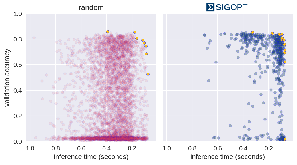
The yellow points in Figure 4 are of interest because no other model configurations are better in both metrics. In academia, the yellow points and their respective hyperparameter configurations are known as Pareto efficient. The collection of each method’s Pareto-efficient points is it’s Pareto frontier. In practice, decision makers allow for some margin of error when calculating the Pareto frontier for multiple objective metrics, as these metrics tend to be noisy when dealing with stochastic model validation techniques.
SigOpt was able to find a better Pareto frontier than random search in ten times fewer evaluations. In fact, when you take the union of both methods’ outputs and examine its Pareto-efficient frontier, SigOpt’s results account for 85.7% of the combined frontier, even though it required 90% fewer model trainings.
Optimizing on a Budget:
The Pareto-Efficient Confidence Region
It took ten times the evaluations—and ten times the computational cost—to reach the fairly sparse frontier given by random search, compared to SigOpt’s dense Pareto frontier. In practice, however, there may be set time and infrastructure constraints at play.
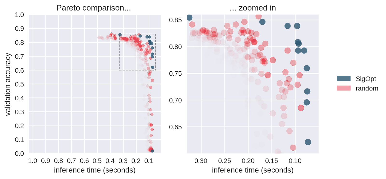
In order to understand what would happen if we allocated the same computational budget to random search as we did to SigOpt, we simulated a confidence region for the Pareto frontier associated with random search on this problem. We subsampled 480 points from the random search, computed the Pareto frontier, repeated this process 800 times and plotted an approximation to the Pareto-efficient confidence region in Figure 5. Areas with higher red intensity imply a higher likelihood of being on the random Pareto frontier.
SigOpt reliably produces better results on both metrics than random search. For example, random search only produced a single point that had a validation accuracy above 0.77 and an inference time below 0.125s. SigOpt’s Pareto frontier has 6 points in this region that all strictly dominate the random search point (as good or better in both metrics). Based on the graph, the points with the highest likelihood of occurring with random search produce a lower accuracy than many of the points of SigOpt’s Pareto frontier. In addition, SigOpt contains many model configurations with inference time half that of the highest likelihood random search points.
Visualization: Intelligent Hyperparameter Tuning
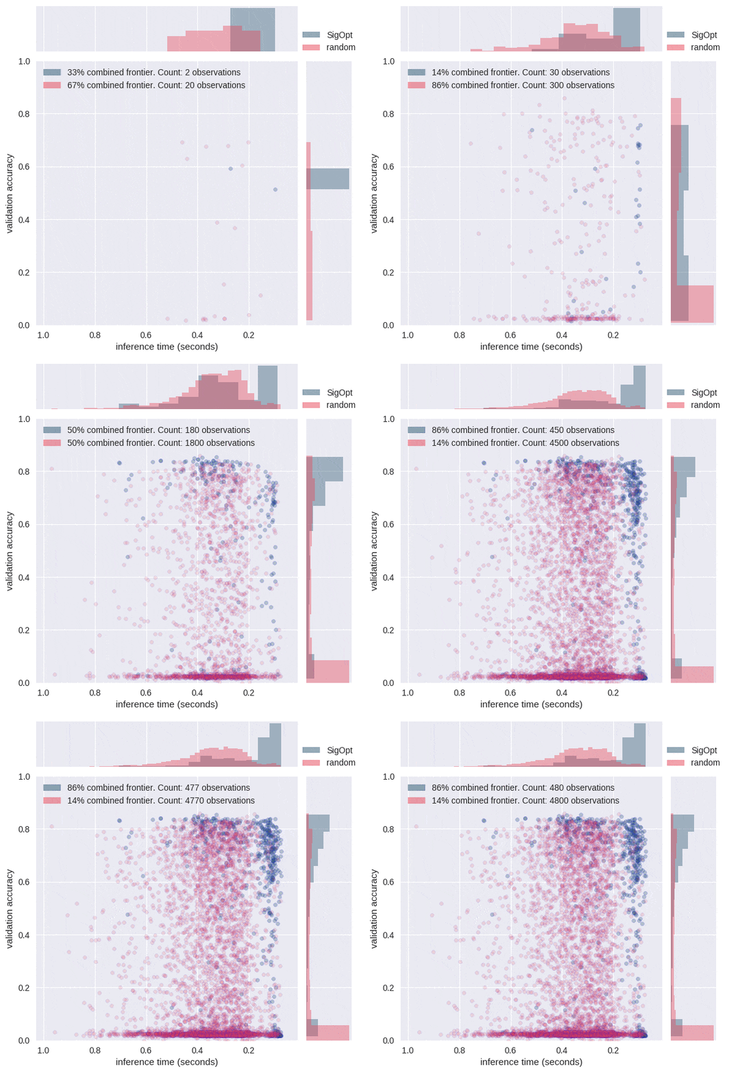
Why does intelligent hyperparameter tuning matter? The animation in Figure 5 shows that SigOpt learns many more efficient hyperparameter configurations than random sampling 10 times as many points, and intelligently learns how to maneuver around the twelve-dimensional hyperparameter space.
Use Case 2: Rotten Tomatoes Sentiment Analysis
As an additional example, we extend a previous post from the AWS AI blog. This example compared hyperparameter optimization strategies for a CNN to maximize model classification accuracy on a natural language processing (NLP) task. Given over 10,000 movie reviews from Rotten Tomatoes, the goal is to create a neural network model that accurately classifies a movie review as either positive or negative.
The Metrics and the Setup
In this experiment we used a MXNet implementation of the convolutional neural network described in [Yoon Kim et al. 2015] for classification of NLP data. Code and instructions for replication of this experiment is available on github here.
Exposing the same hyperparameters as in the AWS post, SigOpt and random search were both used to jointly optimize the metrics of accuracy and training time. SigOpt sampled 480 total hyperparameter configurations, random search sampled 1800 total hyperparameter configurations. All training and inference was performed on AWS P2 instances with a single NVIDIA K80 GPU using the following AMI (ami-193e860f).
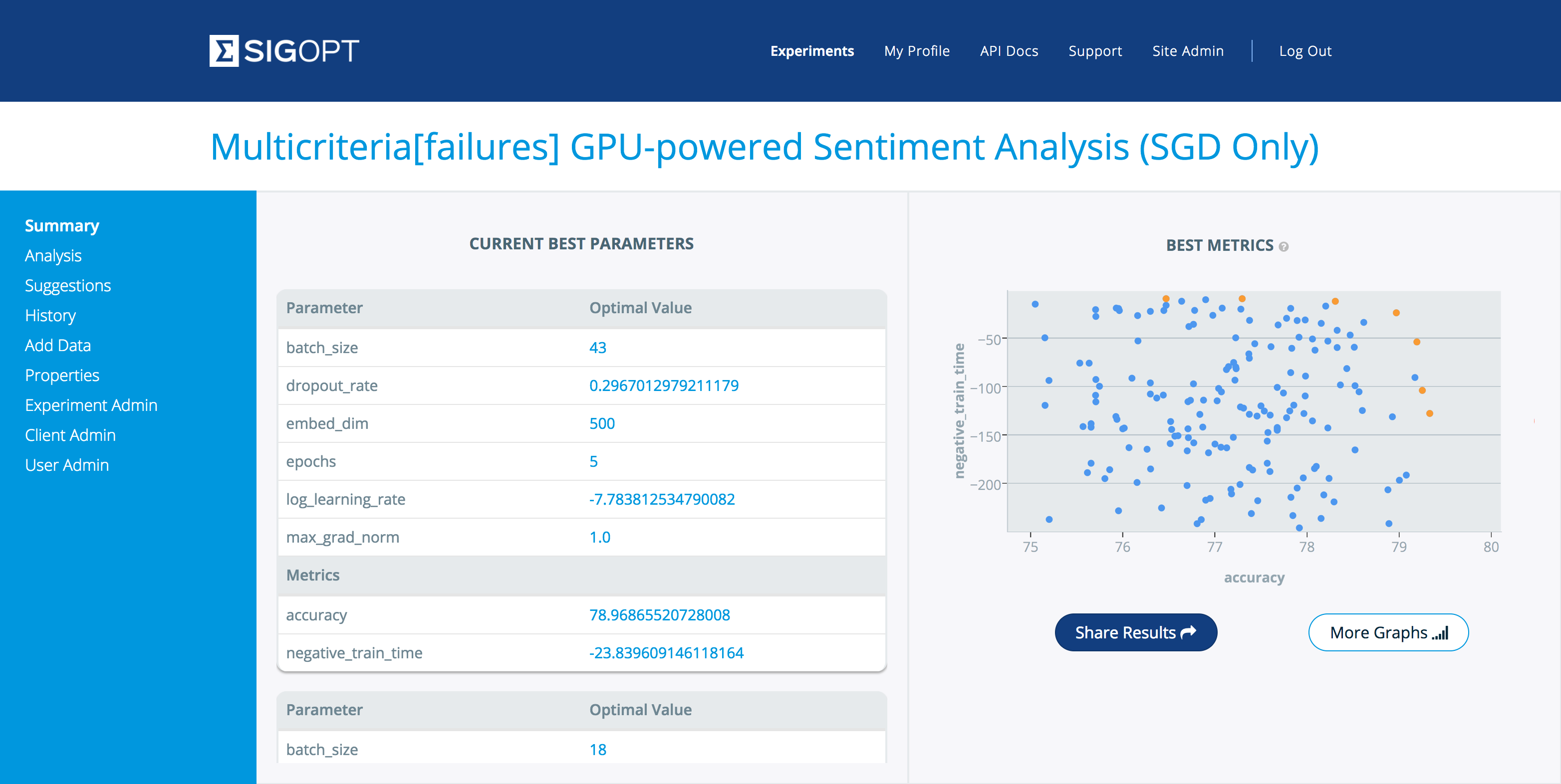
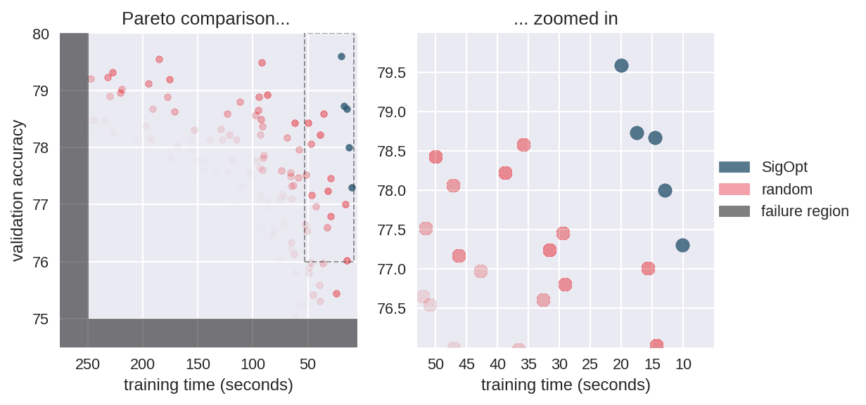
In this example we leverage SigOpt’s ability to learn failure regions in the hyperparameter space. We report model configurations which yield accuracies below 75% and training time over 250 seconds back to SigOpt as failures, forcing the Pareto frontier to be resolved in a focused region shown in Figure 6. This approach could be useful, for example, in a fraud detection pipeline where you may not wish to consider configurations that quickly produce results with lower F-scores than a threshold determined by the business application.
Table 2 shows the six hyperparameters used for this model.
| Hyperparameter | Description |
|---|---|
| embed_dim | Dimensionality of space in which to embed words |
| learning rate | Step size in gradient descent |
| batch_size | Mini-batch size |
| max_grad_norm | Threshold used for gradient clipping |
| epochs | Number of passes through the training data |
| dropout | Fraction of parameter updates to ignore per layer |
Results Overview
As before, we simulated a confidence region for random search’s Pareto frontier as if the budgets were identical, and we see that random search is strictly dominated by SigOpt’s frontier (the SigOpt points are as good, or better, in both metrics). For models that train in less than 250 seconds SigOpt represents 100% of the combined frontier. Employing failure regions helped improve SigOpt’s performance, with 48% of SigOpt’s configurations being in the feasible configuration region and only 26% of random configurations being feasible.
Optimize ML Models Faster with SigOpt
Finding the efficient frontier for your model enables you to choose the best tradeoff between performance metrics given these efficient feasible points. A dense Pareto frontier with higher individual metric values means more and better model configurations to choose from.
Moreover, many modelers with experience in optimization are concerned with the robustness of a solution: when slightly altering a hyperparameter configuration or the underlying data, it is paramount that the model’s performance doesn’t change beyond a small margin of error. While it is the modeler’s responsibility to determine how robust a configuration is, having a dense Pareto frontier with better quality models gives more options for finding an optimally performing robust configuration to deploy into production.
Start Today!
SigOpt enables organizations to get the most from their machine learning pipelines and deep learning models by providing an efficient search of the hyperparameter space leading to better results than traditional methods such as random search, grid search, and manual tuning.
- To replicate the Diatom classification problem, see the github page.
- To replicate the Rotten Tomatoes example, see the github page.
- Visit SigOpt to learn more.
References
[Cornell Computer Science] Movie Review Data
[UC Riverside Computer Science] The UCR Time Series Classification Archive
[Wang et al. 2016] Time Series Classification from Scratch with Deep Neural Networks: A Strong Baseline with Associated Code, Published in IJCNN, 2017, International Joint Conference on Neural Networks, 2017.
[Wang et al. 2015] Imaging Time-Series to Improve Classification and Imputation
[Royal Botanic Garden, Edinburgh] Automatic Diatom Identification and Classification
[Buf and Bayer, 2002] Book on Automatic Diatom Identification
[Jalba, 2004] Automatic Segmentation of Diatom Images for Classification, Microscopy Research and Technique
[Jalba, 2005] Automatic diatom identification using contour analysis by morphological curvature scale spaces, Machine Vision and Applications
[Hu et al. 2013] Time Series Classification under More Realistic Assumptions, SIAM 2013, Data Mining
[Kingma et al. 2015] Adam: A Method For Stochastic Optimization, International Conference on Learning Representations 2015
