
NVIDIA recently announced Morpheus, an AI application framework that provides cybersecurity developers with a highly optimized AI pipeline and pre-trained AI capabilities. Morpheus allows developers for the first time to instantaneously inspect all IP network communications through their data center fabric. Attacks are becoming more and more frequent and dangerous despite the advancements in cybersecurity, and today cybersecurity is mostly reactive. Without real-time AI cybersecurity, companies can resolve problems only after they have already happened. The average time to identify a breach is around 200 days, while remediation of a breach is approximately 70 days.
In part, this is because cybersecurity is a massive data problem. Most companies struggle to monitor all their systems due to the amount of data being generated. Usually they can only sample a small fraction of the total, traditionally at a network perimeter choke point or via low sample rate (SFLOW). Morpheus can help shorten these timeframes by increasing the ability to inspect telemetry from every server at scale and dynamically adapt monitoring based on feedback.
Morpheus includes an optimized AI pipeline and suite of pre-trained AI models. These deep learning and machine learning models can be used in a Morpheus pipeline to accomplish tasks like detecting leaked sensitive information, identifying anomalous behavioral profiles, and detecting suspected phishing attempts. These models are examples, and Morpheus is extensible. Developers and data scientists can deploy their own models using this framework and leverage work they and their organizations have already invested into customized approaches for their unique environments.
In this post, we walk through the Morpheus pipeline and illustrate how to prepare a custom model for Morpheus.
The Morpheus pipeline explained
At its core, Morpheus provides a framework to perform real-time inference across large amounts of telemetry (including raw packet data). This is possible due to the use of GPUs across all parts of the workflow – from data ingestion, into pre-processing, to inference, through post-processing. In addition to faster processing, keeping all of the data on GPU end-to-end eliminates expensive serialization and deserialization actions. But it’s not enough to just focus on raw speed. When inspecting full packet payloads across east/west data center traffic, a larger aperture is needed. GPUs provide massive parallelization that helps move larger volumes of data through the pipeline. By splitting the data and the actions into small batches that are then executed concurrently, Morpheus keeps up with data flowing from heterogeneous sources.
The software stack for Morpheus is shown in Figure 1. Morpheus is built on a number of existing and new technologies, including: RAPIDS, Cyber Log Accelerators (CLX), Triton Inference Server, TensorRT, and cuStreamz. A pub/sub model (currently Kafka) is used to send data to and results from the inference pipeline. These technologies work together to address every part of the cybersecurity workflow:
- RAPIDS and cuStreamz provide accelerated data ingest, pre-processing, and post-processing.
- Triton and TensorRT are used as the inference engines. Since cybersecurity data feeds can sometimes highly vary in size and velocity, Triton’s support for dynamic and ragged batching is very useful.
- CLX includes primitives that are specific to cybersecurity, as well as examples of how to train new models and prepare data for those models.
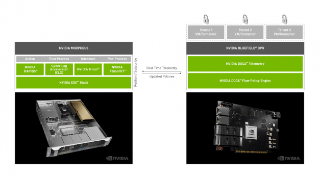
Figure 1: The Morpheus inference pipeline (left side).
Not only can Morpheus perform real-time inference across massive amounts of cybersecurity data, it can also receive network telemetry directly from the NVIDIA BlueField-2 Smart NIC. Telemetry agents running on the NVIDIA DPU route data to Morpheus. For use cases like sensitive information detection and phishing detection, this is often full packet (PCAP) data. But this isn’t a one-way stream. Morpheus produces actions from raw inference results that are passed back to the NIC. These actions allow continuous, real-time, and variable feedback to the NIC that can affect policies, rewrite rules, adjust sensing, and other actions.
The results (actions) from Morpheus are only as effective as the models used. As mentioned earlier, Morpheus comes equipped with several models that can be used to get started. Let’s walk through how one of those models was trained.
How existing Morpheus models are trained
We tend to think about training through two lenses: training from scratch and fine-tuning an existing pre-trained model. While training from scratch gives you ultimate control over every aspect of how a model is trained, it requires a massive amount of labeled training data. While fairly common for image and video domains, this type of training data does not exist for the cybersecurity industry. The onus is therefore on individual organizations to curate these massive datasets.
DIY: Training a DL model in PyTorch for Morpheus
Here we illustrate how to fine-tune an existing BERT model in PyTorch specifically for use in Morpheus. This corresponds roughly to the pre-trained sensitive information detection model. Specifically, this model can identify parts of data such as AWS credentials, GitHub credentials, passwords, and private keys. What makes this approach more powerful than a traditional rules-based approach is that this type of model can generalize. What this means is that we need not expose the model to every possible example during training for it to perform well during inference. We can, for example, train using examples of AWS credentials and not GitHub credentials. But the model will flag on both equally well.
BERT, like many modern NLP models, utilizes a transformer architecture. While this architecture yields incredibly accurate results, the relative complexity of the model sometimes can make inference challenging. Models often need to be especially trained or fine-tuned in order to achieve acceptable results. In order to fine-tune this model, we need some labeled data to adjust the internal weights. Here we assume that that labeled data is extracted and cleaned, and available in a cuDF DataFrame called df. The code below is taken from a full training notebook that illustrates the entire process. Here we focus on the important pieces of code. While this blog talks about sensitive information detection, the Jupyter notebook references PII (Personally Identifying Information) instead. For the purposes of this discussion, they refer to the same fields.
We use DLPack to keep data on the GPU when moving from RAPIDS (cuDF) to PyTorch. No need for expensive copy/converts here.
input_ids, attention_masks = bert_cased_tokenizer(df.text)
labels = from_dlpack(df[label_names].to_dlpack()).type(torch.long)
dataset = TensorDataset(input_ids, attention_masks, labels)

dataset_size = len(input_ids)
train_size = int(dataset_size * .8) # 80/20 split
training_dataset, validation_dataset = random_split(dataset, (train_size, (dataset_size-train_size)))

# create dataloader
train_dataloader = DataLoader(dataset=training_dataset, shuffle=True, batch_size=32)
val_dataloader = DataLoader(dataset=validation_dataset, shuffle=False, batch_size=64)
For this use case, we can actually start with a pre-trained model from the Hugging Face repo. We load that in.
# load pretrained model from transformers repo
model = AutoModelForSequenceClassification.from_pretrained('bert-base-cased', num_labels=num_labels)
model.cuda();
model.train();
If more than one GPU is available, we can further parallelize using the DataParallel method in PyTorch. This distributes the data across multiple GPUs.
# find number of gpus
n_gpu = torch.cuda.device_count()

# use DataParallel if you have more than one GPU
if n_gpu > 1:
    model = torch.nn.DataParallel(model)

# number of training epochs
epochs = 4
The main training loop is where the fine-tuning happens. It’s during this phase that the internal weights of the neural network are updated. In addition, a classification layer is added that performs the final step of the sequence labeling task.
# train loop
for _ in trange(epochs, desc="Epoch"):
    # tracking variables
        tr_loss = 0 #running loss
        nb_tr_examples, nb_tr_steps = 0, 0

    # train the data for one epoch
    for batch in train_dataloader:
        # unpack the inputs from dataloader
        b_input_ids, b_input_mask, b_labels = batch

        # clear out the gradients
        optimizer.zero_grad()

        # forward pass
        outputs = model(b_input_ids, attention_mask=b_input_mask)
        logits = outputs[0]

        # using binary cross-entropy with logits as loss function
        # assigns independent probabilities to each label
        loss_func = BCEWithLogitsLoss()

        # convert labels to float for calculation
        loss = loss_func(logits.view(-1,num_labels),b_labels.type_as(logits).view(-1,num_labels))

        # mean() to average on multi-gpu parallel training
        if n_gpu > 1:
            loss = loss.mean()

        # backward pass
        loss.backward()

        # update parameters and take a step using the computed gradient
        optimizer.step()

        # update tracking variables
        tr_loss += loss.item()
        nb_tr_examples += b_input_ids.size(0)
        nb_tr_steps += 1

    print("Train loss: {}".format(tr_loss/nb_tr_steps)
Evaluating the model for accuracy is important, and the full example of how to do that is in the linked notebook, just scroll down to the evaluation section near the bottom. Calculating the macro-F1 score is one way to evaluate the model, but since we’re using this to identify many different types of sensitive information (some perhaps more sensitive than others), we may care about the accuracy of each class. Calculating the full confusion matrix for each label is one way to gain insight into the model’s performance at a finer granularity.
Once you’re happy with the model and its performance, it can be saved to disk.
# save out the model
if n_gpu > 1:
    torch.save(model.module.state_dict(), "path/to/your-model-name.pth")
else:
    torch.save(model.state_dict(), "path/to/your-model-name.pth")
Moving the model to ONNX
Once a model is performing according to expectations, it’s easy to get it into ONNX. ONNX (the Open Neural Network Exchange format) is a common format for neural networks that enable cross framework and tool compatibility. Triton is built in such a way that it is easy to swap backends (and even write your own if you prefer), and the ONNX runtime is one of those existing backends (with support for v1.4 as of this post).
Using a PyTorch model named torch_model, it’s fairly straightforward to get that model into ONNX. The variable model_input refers to some test data. Because the command to export to ONNX runs the model, this input is required. The values can be random as long as the data is the right type and size.
import torch.onnx
torch.onnx.export(torch_model, model_input,

    # where to save the model
    "bert-model-seq-len-256.onnx",

    # store the trained parameter weights inside the model file
    export_params=True,

    # the ONNX version to export the model to
    opset_version=10,

    # whether to execute constant folding for optimization
    do_constant_folding=True,

    # the model's input names
    input_names = ['input_ids','attention_mask'],

    # the model's output names
        output_names = ['output'],

    # variable length axes
    dynamic_axes={'input_ids' : {0 : 'batch_size'},
                  'attention_mask': {0: 'batch_size'},
                  'output' : {0 : 'batch_size'}})
The output here is the bert-model-seq-len-256.onnx file that can now be integrated into Morpheus.
Deploying your model in Morpheus
Morpheus provides a wrapper to import your model into a pipeline.
python cli.py onnx-to-trt    \
    --input_model=.tmp/models_onnx/bert-model-seq-len-256.onnx  \
    --output_model=.tmp/models_onnx/bert-model-256seq_b1-8_b1-16.engine  \
    --batches 1 8 \
    --batches 1 16 \
    --seq_length=256
This imports the ONNX model bert-model-seq-len-256.onnx into the inference pipeline. Under the hood, this wrapper performs some heavy lifting – including optimizing the model for TensorRT and serializing this high-performance, highly tuned version. Morpheus abstracts all of that away from the user and lets them focus on deploying their model in a single command. Once the model is deployed to Morpheus, the pipeline is ready for inferencing to run.
There are several ways to get data into and out of Morpheus, including the NetQ telemetry agent running on the BlueField 2 DPU. But interfacing with Kafka is also supported, both for data ingest as well as collecting results after inference. Making these connections is straightforward, supplying the broker and topics to be used for data ingest as well as the topics for publishing results.
Next steps
We’re just scratching the surface with Morpheus. In addition to future pre-trained models, the first release of Morpheus will integrate MLFlow, bringing an even easier to use method to manage, update and track models. While inference speeds are already high, work is continuing to optimize models for higher throughput, identify and optimize bottlenecks in the pipeline, and create training scripts that anyone can use to build custom models. Figure 2 shows the speedup of the optimized end-to-end Morpheus pipeline over a baseline that simply runs in PyTorch – showing an increase in throughput by over 125x.
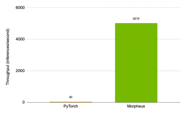
Figure 2: Speedup of the Morpheus pipeline over an unoptimized one.
AI will be a critical tool to help fight cybercrime more effectively in the future and will demand new levels of computing and scale. Morpheus is the framework that will enable application developers and the security ecosystem to meet the challenges of securing modern networks against sophisticated attacks. Apply for early access to Morpheus, and get started with it when available in June 2021.
