
You could make an argument that the history of civilization and technological advancement is the history of the search and discovery of materials. Ages are named not for leaders or civilizations but for the materials that defined them: Stone Age, Bronze Age, and so on. The current digital or information age could be renamed the Silicon or Semiconductor Age and retain the same meaning.
Though silicon and other semiconductor materials may be the most significant materials driving change today, there are several other materials in research that could equally drive the next generation of changes, including any of the following:
- High-temperature superconductors
- Photovoltaics
- Graphene batteries
- Supercapacitors
Semiconductors are at the heart of building chips that enable the extensive and computationally complex search for such novel materials.
In 2011, the United States’ Materials Genome Initiative pushed for the identification of new materials using simulation. However, at that time and to an extent even today, calculating material properties from first principles can be painfully slow even on modern supercomputers.
The Vienna Ab initio Simulation Package (VASP) is one of the most popular software tools for such predictions, and it has been written to leverage acceleration technologies and to minimize the time to insight.
New material review: Hafnia
This post examines the computation of the properties of a material called hafnia or hafnium oxide (HfO2).
On its own, hafnia is an electric insulator. It is heavily used in semiconductor manufacturing, as it can serve as a high-κ dielectric film when building dynamic random-access memory (DRAM) storage. It can also act as a gate insulator in metal–oxide–semiconductor field-effect transistors (MOSFETs). Hafnia is of high interest for nonvolatile resistive RAM, which could make booting computers a thing of the past.
While an ideal, pure HfO2 crystal can be calculated affordably using only 12 atoms, it is nothing but a theoretical model. Such crystals have impurities in practice.
At times, a dopant must be added to yield the desired material properties beyond insulation. This doping can be done at the purity level, which means that out of 100 eligible atoms, one atom is replaced by a different element. There are minimally 12 atoms out of which only four are Hf. It soon becomes apparent that such calculations easily call for hundreds of atoms.
This post demonstrates how such calculations can be parallelized efficiently over hundreds and even thousands of GPUs. Hafnia serves as an example, but the principles demonstrated here can of course be applied to similarly sized calculations just as well.
Term definitions
- Speedup: A nondimensional measure of performance relative to a reference. For this post, the reference is single-node performance using 8x A100 80 GB SXM4 GPUs without NCCL enabled. Speedup is calculated by dividing the reference runtime by the elapsed runtime.
- Linear scaling: The speedup curve for an application that is perfectly parallel. In Amdahl’s law terms, it is for an application that is 100% parallelized and the interconnect is infinitely fast. In such a situation, 2x the compute resources results in half the run time and 10x the compute resources results in one-tenth the run time. When plotting speedup compared to number of compute resources, the performance curve is a line sloping up and to the right at 45 degrees. The effect of a parallelized run outperforms this proportional relation. That is, the slope would be steeper than 45 degrees and it is called super-linear scaling.
- Parallel efficiency: A nondimensional measure in percent of how close a particular application execution is to the ideal linear scaling. Parallel efficiency is calculated by dividing the achieved speedup by the linear scaling speedup for that number of compute resources. To avoid wasting compute time, most data centers have policies on minimum parallel efficiency targets (50-70%).
VASP use cases and differentiation
VASP is one of the most widely used applications for electronic-structure calculations and first-principles molecular dynamics. It offers state-of-the-art algorithms and methods to predict material properties like the ones discussed earlier.
The GPU acceleration is implemented using OpenACC. GPU communications can be carried out using the Magnum IO MPI libraries in NVIDIA HPC-X or NVIDIA Collective Communications Library (NCCL).
Use cases and differentiation of hybrid DFT
This section focuses on using a quantum-chemical method known as density functional theory (DFT) that reaches higher-accuracy predictions by mixing in exact-exchange calculations to approximations within the DFT and is then called hybrid DFT. This added accuracy helps to determine band gaps in closer accordance with experimental results.
Band gaps are the property that classifies materials as insulators, semiconductors, or conductors. For materials based on hafnia, this extra accuracy is crucial, but comes at an increased computational complexity.
Combining this with the need for using many atoms demonstrates the demand for scaling to many nodes on GPU-accelerated supercomputers. Fortunately, even higher accuracy methods are available in VASP. For more information about the additional features, see VASP6.
At a higher level, VASP is a quantum-chemistry application that is different from other, and possibly even more familiar, high-performance computing (HPC) computational-chemistry applications like NAMD, GROMACS, LAMMPS, and AMBER. These codes focus on molecular dynamics (MD) using simplifications to the interactions between atoms such as treating them as point charges. This makes simulations of the movement of those atoms, say because of temperature, computationally inexpensive.
VASP, on the other hand, treats the interaction between atoms on the quantum level, in that it calculates how the electrons interact with each other and can form chemical bonds. It can also derive forces and move atoms for a quantum or ab-initio-MD (AIMD) simulation. This can indeed be interesting to the scientific problem discussed in this post.
However, such a simulation would consist of repeating the hybrid-DFT calculation step many times. While subsequent steps might converge faster, the computational profile of each individual step would not change. This is why we only show a single, ionic step here.
Running single-node or multi-node
Many VASP calculations employ chemical systems that are small enough not to require execution on HPC facilities. Some users might be uncomfortable with scaling VASP on multiple nodes and suffer through the time-to-solutions, maybe even to the extent that a power outage or some other failure becomes probable. Others may limit their simulation sizes so that runtimes are not as onerous as they would be if better-suited system sizes were investigated.
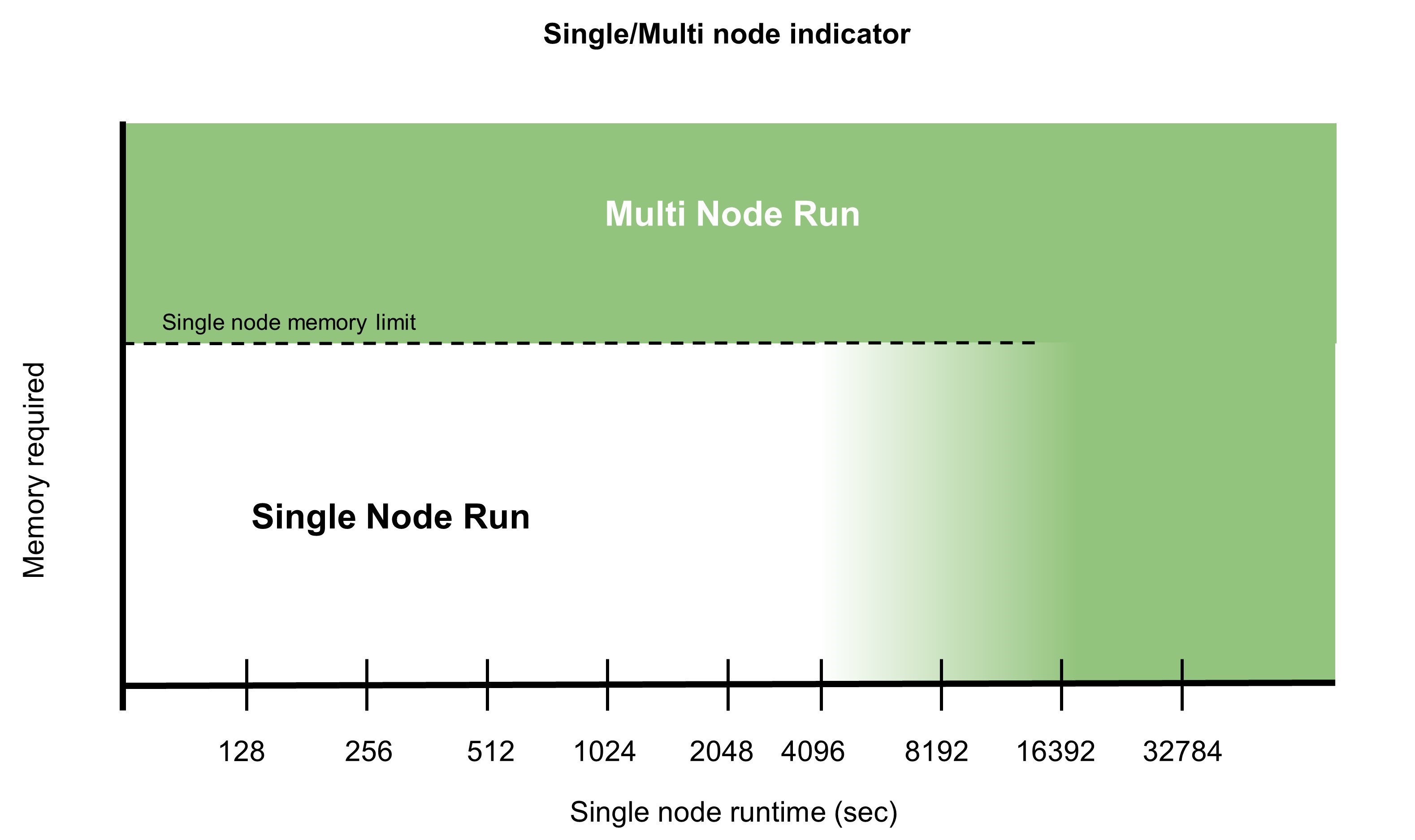
There are multiple reasons that would drive you toward running simulations multi-node:
- Simulations that would take an unacceptable amount of time to run on a single node, even though the latter might be more efficient.
- Large calculations that require large amounts of memory and cannot fit on a single node require distributed parallelism. While some computational quantities must be replicated across the nodes, most of them can be decomposed. Therefore, the amount of memory required per node is cut roughly by the number of nodes participating in the parallel task.
For more information about multi-node parallelism and compute efficiency, see the recent HPC for the Age of AI and Cloud Computing ebook.
NVIDIA published a study of multi-node parallelism using the dataset Si256_VJT_HSE06. In this study, NVIDIA asked the question, “For this dataset, and an HPC environment of V100 systems and InfiniBand networking, how far can we reasonably scale?”
Magnum IO communication tools for parallelism
VASP uses the NVIDIA Magnum IO libraries and technologies that optimize multi-GPU and multi-node programming to deliver scalable performance. These are part of the NVIDIA HPC SDK.
In this post, we look at two communication libraries:
- Message Passing Interface (MPI): The standard for programming distributed-memory scalable systems.
- NVIDIA Collective Communications Library (NCCL): Implements highly optimized multi-GPU and multi-node collective communication primitives using MPI-compatible all-gather, all-reduce, broadcast, reduce, reduce-scatter, and point-to-point routines to take advantage of all available GPUs within and across your HPC server nodes.
VASP users can choose at runtime what communication library should be used. As performance most often improves significantly when MPI is replaced with NCCL, this is the default in VASP.
There are a couple of strong reasons for the observed differences when using NCCL over MPI.
With NCCL, communications are GPU-initiated and stream-aware. This eliminates the need for GPU-to-CPU synchronization, which is otherwise needed before each CPU-initiated MPI communication to ensure that all GPU operations have completed before the MPI library touches the buffers. NCCL communications can be enqueued on a CUDA stream just like a kernel and can facilitate asynchronous operation. The CPU can enqueue further operations to keep the GPU busy.
In the MPI case, the GPU is idle at least for the time that it takes the CPU to enqueue and launch the next GPU operation after the MPI communication is done. Minimizing GPU idle times contributes to higher parallel efficiencies.
With two separate CUDA streams, you can easily use one stream to do the GPU computations and the other one to communicate. Given that these streams are independent, the communication can take place in the background and potentially be hidden entirely behind the computation. Achieving the latter is a big step forward to high parallel efficiencies. This technique can be used in any program that enables a double-buffering approach.
Nonblocking MPI communications can expose similar benefits. However, you still must handle the synchronizations between the GPU and CPU manually with the described performance downsides.
There is another layer of complexity added as the nonblocking MPI communications must be synchronized on the CPU side as well. This requires much more elaborate code from the outset, compared to using NCCL. However, with MPI communications being CPU-initiated, there often is no hardware resource that automatically makes the communications truly asynchronous.
You can spawn CPU threads to ensure communications progress if your application has CPU cores to spend, but that again increases code complexity. Otherwise, the communication might only take place when the process enters MPI_Wait, which offers no advantage over using blocking calls.
Another difference to be aware of is that for reductions, the data is summed up on the CPU. In the case where your single-threaded CPU memory bandwidth is lower than the network bandwidth, this can be an unexpected bottleneck as well.
NCCL, on the other hand, uses the GPU for summations and is aware of the topology. Intranode, it can use available NVLink connections and optimizes internode communication using Mellanox Ethernet, InfiniBand, or similar fabrics.
Computational modeling test case with HfO2
A hafnia crystal is built from two elements: hafnium (Hf) and oxygen (O). In an ideal system free from dopants or vacancies, for each Hf atom, there will be two O atoms. The minimum number of atoms to describe the structure of the infinitely extended crystal required is four Hf (yellowish) and eight O (red) atoms. Figure 2 shows the structure.
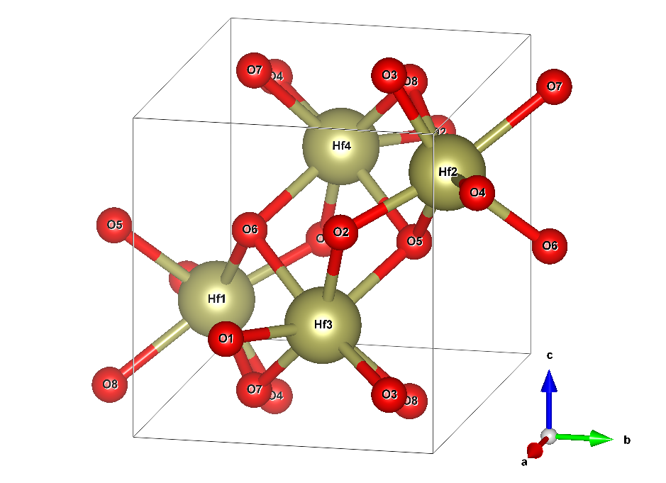
The box wireframe designates the so-called unit cell. It is repeated in all three dimensions of space to yield the infinitely extended crystal. The picture alludes to that by duplicating the atoms O5, O6, O7, and O8 outside of the unit cell to show their respective bonds to the Hf atoms. This cell has a dimension of 51.4 by 51.9 by 53.2 nm. This is not a perfect cuboid because one of its angles is 99.7° instead of 90°.
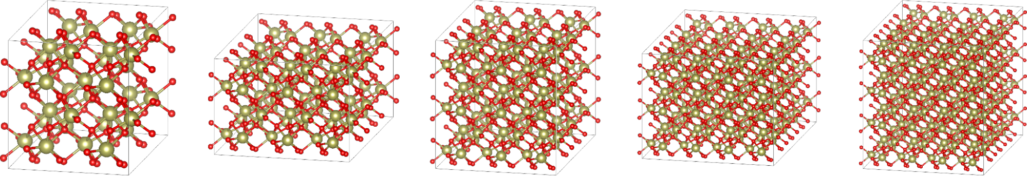
The minimal model only treats the 12 atoms enclosed in the box in Figure 2 explicitly. However, you can also prolong the box in one or more directions of space by an integer multiple of the according edge and copy the structure of atoms into the newly created space. Such a result is called a supercell and can help to treat effects that are inaccessible within the minimal model, like a 1% vacancy of oxygen.
Of course, treating a larger cell with more atoms is computationally more demanding. When you add one more cell, so that there are two total cells, in the direction of a while leaving b and c as is, this is called a 2x1x1 supercell with 24 atoms.
For the purposes of this study, we only considered supercells that are costly enough to justify the usage of at least a handful of supercomputer nodes:
- 2x2x2: 96 atoms, 512 orbitals
- 3x3x2: 216 atoms, 1,280 orbitals
- 3x3x3: 324 atoms, 1,792 orbitals
- 4x4x3: 576 atoms, 3,072 orbitals
- 4x4x4: 768 atoms, 3,840 orbitals
Keep in mind that computational effort is not directly proportional to the number of atoms or the volume of the unit cell. A rough estimate used in this case study is that it scales cubically with either.
The hafnia system used here is only one example, of course. The lessons are transferable to other systems that employ similar-sized cells and hybrid DFT as well because the underlying algorithms and communication patterns do not change.
If you want to do some testing yourself with HfO2, you can download the input files used for this study. For copyright reasons, we may not redistribute the POTCAR file. This file is the same across all supercells. As a VASP licensee, you can easily create it yourself from the supplied files by the following Linux command:
# cat PAW_PBE_54/Hf_sv/POTCAR PAW_PBE_54/O/POTCAR > POTCAR
For these scaling experiments, we enforced a constant number of employed crystal orbitals, or bands. This slightly increases the workload beyond the minimum required but has no effect on computational accuracy.
If this wasn’t done, VASP would automatically select a number that is integer-divisible by the number of GPUs and this might increase the workload for certain node counts. We chose the number of orbitals that is integer-divisible by all GPU counts employed. Also, for better computational comparability, the number of k-points is kept fixed at 8, even though larger supercells might not require this in practice.
Supercell modeling test method with VASP
All benchmarks presented in the following are using the latest VASP release 6.3.2, which was compiled using the NVIDIA HPC SDK 22.5 and CUDA 11.7.
For full reference, makefile.include is available for download. They were run on the NVIDIA Selene supercomputer that consists of 560 DGX A100 nodes, each of which provides eight NVIDIA A100-SXM4-80GB GPUs, eight NVIDIA ConnectX-6 HDR InfiniBand network interface cards (NICs), and two AMD EPYC 7742 CPUs.
To ensure the best performance, the processes and threads were pinned to the NUMA nodes on the CPU that offer ideal connectivity to the respective GPUs and NICs that they will use. The reverse NUMA node numbering on AMD EPYC, yields the following process binding for the best hardware locality.
| Node local rank | CPU NUMA node | GPU ID | NIC ID |
| 0 | 3 | 0 | mlx5_0 |
| 1 | 2 | 1 | mlx5_1 |
| 2 | 1 | 2 | mlx5_2 |
| 3 | 0 | 3 | mlx5_3 |
| 4 | 7 | 4 | mlx5_6 |
| 5 | 6 | 5 | mlx5_7 |
| 6 | 5 | 6 | mlx5_8 |
| 7 | 4 | 7 | mlx5_9 |
Included in the set of downloadable files is a script called selenerun-ucx.sh. This script is wrapping the call to VASP by performing the following in the workload manager (for example, Slurm) job script:
# export EXE=/your/path/to/vasp_std
# srun ./selenerun-ucx.sh
The selenerun-ucx.sh file must be customized to match your environment, depending on the resource configuration available. For example, the number of GPUs or number of NICs per node may be different from Selene and the script must reflect those differences.
To keep computation time for benchmarking as low as possible, we have restricted all calculations to only one electronic step by setting NELM=1 in the INCAR files. We can do this because we are not concerned with the scientific results like the total energy and running one electronic step suffices to project the performance of a full run. Such a run took 19 iterations to converge with the 3x3x2 supercell.
Of course, each different cell setup could require a different number of iterations until convergence. To benchmark scaling behavior, you want to compare fixed numbers of iterations anyway to keep the workload comparable.
However, evaluating the performance of runs with only one electronic iteration would mislead you because the profile is lopsided. Initialization time would take a much larger share relative to the net iterations and so would the post-convergence parts like the force calculation.
Luckily, the electronic iterations all require the same effort and time. You can project the total runtime of a representative run using the following equation:
\(t_{total} = t_{init} + 19 \cdot t_{iter} +t_{post}\)
You can extract the time for one iteration \(t_{init}\) from the VASP internal LOOP timer, while the time spent in post-iteration steps \(t_{post}\) is given by the difference between the LOOP+ and LOOP timers.
The initialization time \(t_{init}\), on the other hand, is the difference between the total time reported in VASP as Elapsed time and LOOP+. There is a slight error in such a projection as the first iterations take a little longer due to instances such as one-time allocations. However, the error was checked to be less than 2%.
Parallel efficiency results for a hybrid DFT iteration in VASP
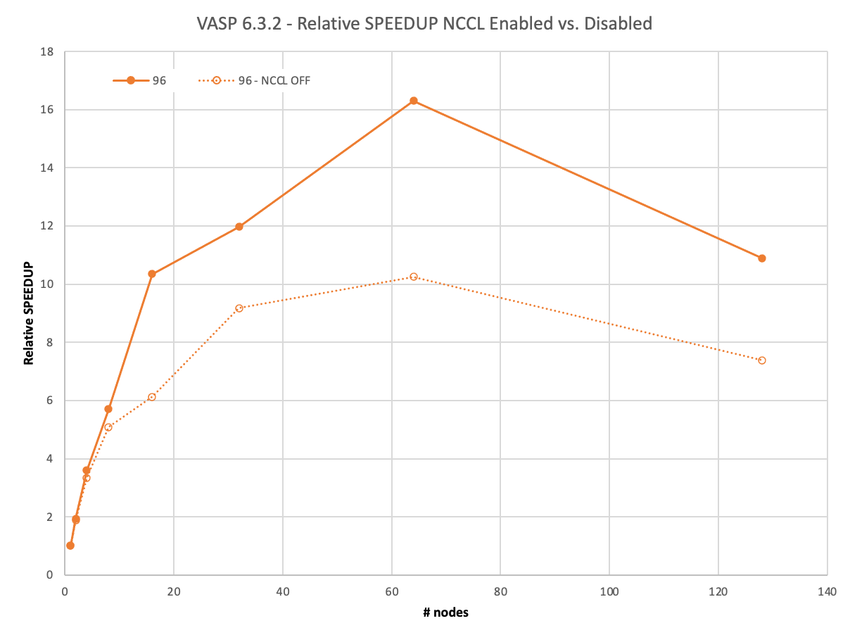
We first reviewed the smallest dataset with 96 atoms: the 2x2x2 supercell. This dataset hardly requires a supercomputer these days. Its full run, with 19 iterations, finishes in around 40 mins on one DGX A100.
Still, with MPI, it can scale to two nodes with 93% parallel efficiency before dropping to 83% on four and even 63% on eight nodes.
On the other hand, NCCL enables nearly ideal scaling of 97% on two nodes, 90% on four nodes, and even on eight nodes it still reaches 71%. However, the biggest advantage by NCCL is clearly demonstrated at 16 nodes. You can still see a >10x relative speedup compared to 6x with MPI only.
The negative scaling beyond 64 nodes needs explanation. To run 128 nodes with 1024 GPUs, you must use 1024 orbitals as well. The other calculations used only 512, so here the workload increases. We didn’t want to include such an excessive orbital count for the lower node runs, though.
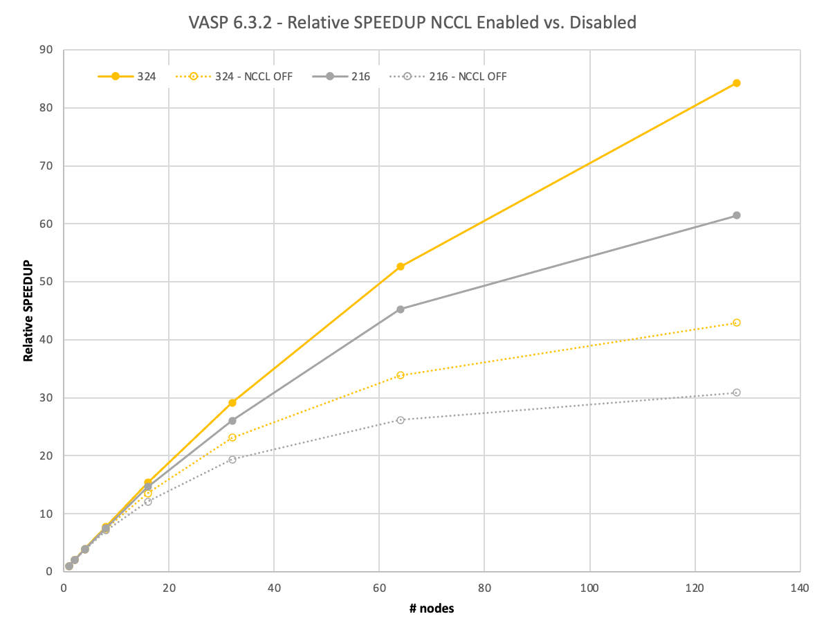
The next example is already a computationally challenging problem. The full calculation of the 3x3x2 supercell featuring 216 atoms takes more than 7.5 hours to complete on 8xA100 on a single node.
With more demand on computation, there is more time to conclude the communications asynchronously in the background using NCCL. VASP remains above 91% until 16 nodes and only closely falls short of 50% on 128 nodes.
With MPI, VASP does not hide the communications effectively and does not reach 90% even on eight nodes and drops to 41% on 64 nodes already.
Figure 5 shows that the trends regarding the scaling behavior remain the same for the next bigger 3x3x3 supercell with 324 atoms, which would take a full day until the solution on a single node. However, the spreads between using NCCL and MPI increase significantly. On 128 nodes with NCCL, you gain a 2x better relative speedup.
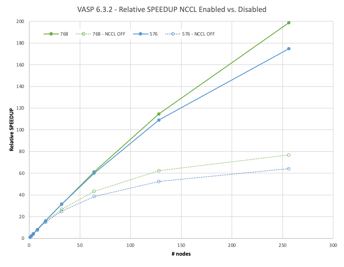
Going to an even larger, 4x4x3 supercell containing 576 atoms, you would have to wait more than 5 days for the full calculation using one DGX A100.
However, with such a demanding dataset, a new effect must be discussed: Memory capacity and parallelization options. VASP offers to distribute the workload over k-points while replicating the memory in such setups. While this is much more effective for standard-DFT runs, it also helps with performance on hybrid-DFT calculations and there is no need to leave available memory unused.
For the smaller datasets, even parallelizing over all k-points fits easily into 8xA100 GPUs with 80 GB of memory each. With the 576-atom dataset, on a single node, this is no longer the case though and we must reduce the k-point parallelism. From two nodes onwards, we could fully employ it again.
While it is indistinguishable in Figure 6, there is minor super-linear scaling in the MPI case (102% parallel efficiency) on two nodes. This is because of the necessarily reduced parallelism on one node that is lifted on two or more nodes. However, that is what you would do in practice as well.
We face a similar situation for the 4x4x4 supercell with 768 atoms on one and two nodes, but the super-linear scaling effect is even less pronounced there.
We scaled the 4x4x3 and 4x4x4 supercell to 256 nodes. This equates to 2,048 A100 GPUs. With NCCL, they achieved 67% or even 75% of parallel efficiency. This enables you to yield your results in less than 1.5 hours, in what would have previously taken almost 12 days on one node! The usage of NCCL enables an almost 3x higher relative speedup for such large calculations over MPI.
Recommendations for using NCCL for a VASP simulation
VASP 6.3.2 calculating HfO2 supercells ranging from 96 to 768 atoms achieves significant performance by using NVIDIA NCCL across many nodes when an NVIDIA GPU-accelerated HPC environment enhanced by NVIDIA InfiniBand networking is available.
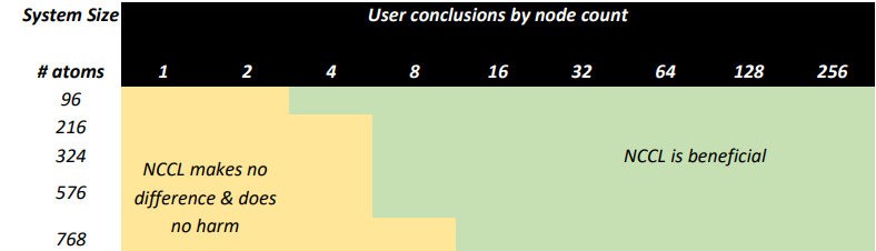
Based on this testing, we recommend that users with access to capable HPC environments consider the following:
- Run all but the smallest calculations using GPU acceleration.
- Consider running larger systems of atoms using both GPUs and multiple nodes to minimize time to insight.
- Launch all multi-node calculations using NCCL as it only increases efficiency when running large models.
The slight added overhead to initialize NCCL will be worth the tradeoff.
Summary
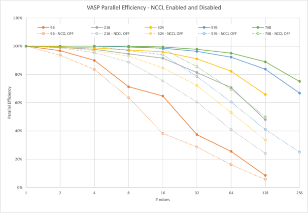
In conclusion, you’ve seen that scalability for hybrid DFT in VASP depends on the size of the dataset. This is somewhat expected given that the smaller the dataset is, the earlier each individual GPU will run out of computational load.
NCCL also helps to hide the required communications. Figures 7 and 8 show the levels of parallel efficiency that you can expect for certain dataset sizes with varying node counts. For most computationally intensive datasets, VASP reaches >80% of parallel efficiency on 32 nodes. For the most demanding datasets, as some of our customers request them, scale-out runs at 256 nodes are possible with good efficiency.
VASP user experience
From our experience with VASP users, running VASP on GPU-accelerated infrastructure is a positive and productive experience that enables you to consider larger and more sophisticated models for your research.
In unaccelerated scenarios, you may be running models smaller than you’d like because you expect runtimes to grow to intolerable levels. Using high-performance, low-latency I/O infrastructure with GPUs, and InfiniBand with Magnum IO acceleration technologies like NCCL, makes efficient, multi-node parallel computing practical and puts larger models within reach for investigators.
HPC system administrator benefits
HPC centers, especially commercial ones, often have policies that prohibit users from running jobs at low parallel efficiency. This prevents users on short deadlines or who need high turn-over rates from using more computational resources at the expense of other users’ job wait time. More often than not, a simple rule of thumb is that 50% parallel efficiency dictates the maximum number of nodes that a user might request and hence increases the time to solution.
We have shown here that, by using NCCL as part of NVIDIA Magnum IO, users of an accelerated HPC system can stay well within efficiency limits and scale their jobs significantly farther than possible when using MPI alone. This means that while keeping overall throughput at its highest across the HPC system, you can minimize runtime and maximize the number of simulations to get new and exciting science done.
HPC application developer advantages
As an application developer, you can benefit from the advantages observed here with VASP just as well. To get started:
- Download NCCL.
- Read the NCCL User Guide.
- Review the popular Fast Inter-GPU Communication with NCCL for Deep Learning Training, and More (a Magnum IO session) GTC session.
- Read these informative posts:
