Optimize Energy Efficiency of Multi-Node VASP Simulations with NVIDIA Magnum IO

Computational energy efficiency has become a primary decision criterion for most supercomputing centers. Data centers, once built, are capped in terms of the amount of power they can use without expensive and time-consuming retrofits. Maximizing insight in the form of workload throughput then means maximizing workload per watt. NVIDIA products have, for several generations, focused on maximizing real application performance per kilowatt hour (kWh) used.

This post explores measuring and optimizing energy usage of multi-node hybrid density functional theory-(DFT) calculations with the Vienna Ab initio Simulation Package (VASP). VASP is a computer program for atomic-scale materials modeling, such as electronic structure calculations and quantum-mechanical molecular dynamics, from first principles.

Material property research is an active area for researchers using supercomputing facilities for cases as broad as high-temperature, low-pressure superconductors, to the next generation of solar cells. VASP is a primary tool in these digital investigations.

This post follows our 2022 investigation on multi-node VASP scalability for varying system sizes of a simple compound hafnia (HfO₂). For details, see Scaling VASP with NVIDIA Magnum IO.

Experiment setup

The environment and setup used for this energy-focused extension of our previous work is largely the same. This section provides details about our experiment setup for reproducing our results.

Hardware: NVIDIA GPU system

NVIDIA Selene cluster
NVIDIA DGX A100
AMD EPYC 7742 64C 2.25 GHz
NVIDIA A100 Tensor Core GPUs (80 GB) (eight per node)
NVIDIA HDR InfiniBand (eight per node)

Hardware: CPU system

Dual-socket Intel 8280 CPUs (28 cores per socket)
192 GB per node
NVIDIA HDR InfiniBand per node

Software

Updated versions for all the following components of the NVIDIA GPU software stack are available. However, we intentionally used the same components as for our previous work to retain comparability. VASP was updated to version 6.4 released in 2023.

NVIDIA HPC SDK 22.5 (formerly known as PGI)
NVIDIA Magnum IONCCL 2.12.9
CUDA 11.7
FFT
- GPU: FFT lib – cuFFT 10.7.2 (GPU side)
- CPU: FFTW interface comes from Intel MKL 2020.0.166
MPI: open MPI 4.1.4rc2 compiled with PGI
UCX
VASP 6.4.0

For runs on an Intel CPU-only cluster, we employed the accordingly optimal toolchain consisting of the most recent version available at the time of writing:

Rocky Linux release 9.2 (Blue Onyx)
Intel oneAPI HPC Toolkit 2022.3.1
MPI: hpcx-2.15

Extrapolating runtime and energy

As detailed in Scaling VASP with NVIDIA Magnum IO, we shortened the benchmarking runs and extrapolated to the full results to save resources. In other words, we only used a fraction of the energy presented in the following formula:

$t_{total} = t_{init} + 19 t_{iter} + t_{post}$

The method was extended for energy by assuming the energy used for one iteration was similarly constant:

$E_{total} = E_{init} + 19 E_{iter} + E_{post}$

Chemistry and models

Chemistry: hafnia (HfO₂)
Models:
- 3x3x2: 216 atoms, 1,280 orbitals
- 3x3x3: 324 atoms, 1,792 orbitals
- 4x4x3: 576 atoms, 3,072 orbitals
- 4x4x4: 768 atoms, 3,840 orbitals

Capturing energy usage

The GPU benchmarks were done on the NVIDIA Selene supercomputer, which is equipped with smart PDUs that can provide information on currently used power through the SNMP protocol. We collected the data using a simple Python script launched in the background of each node before starting the application.

We collected ‌power usage with a frequency of 1 Hz combined with timestamps. Given that, for GPU runs at hybrid-DFT level, VASP leaves the CPU mostly idle, this logging comes at almost no overhead. Based on the information in the files and timestamps included in the outputs from VASP, we calculated the energy usage for each part of the code and project as described above.

Optimizing for best energy efficiency (MaxQ)

By default, NVIDIA GPUs operate at their maximum clock frequency with sufficient load to ensure best possible performance, and hence time to solution. However, the performance of certain parts of an application might not be primarily limited by clock frequency to begin with.

Higher clock frequencies require higher voltages, and this in turn leads to a higher energy uptake. Hence, the sweet spot for the maximum GPU clock frequency for solving a problem in the shortest time to solution might be different from those necessary to achieve the lowest energy to solution.

Looking at hypothetical applications that are entirely limited by memory loads and stores, one would expect the lowest frequency that suffices to still saturate memory bandwidth should give a better energy to solution while not impairing performance.

Given that real applications have mixed computational profiles and the dependence on frequency varies with the workload, the ideal frequency can be determined on a case-by-case basis. This was done for the VASP hafnia workloads presented here. However, we ‌have observed that our findings also work well for other high-performance computing (HPC) applications.

The frequencies can be controlled through the NVIDIA System Management Interface (SMI), as shown in the code snippets below:

-lgc --lock-gpu-clocks= Specifies <minGpuClock,maxGpuClock> clocks as a pair (1500,1500) that defines
the range of desired locked GPU clock speed in MHz. 
Setting this will supersede application clocks and take effect regardless if an app is running. 
Input can also be a singular desired clock value (<GpuClockValue>).

For example:
# nvidia-smi -pm 1
# nvidia-smi -i 0 -pl 250
# nvidia-smi -i 0 -lgc 1090,1355

Additional data collected includes:

CPU multi-node performance
Single-node, SM frequency sweep for MaxQ

Results

This section showcases the influence of GPU clock frequency on energy usage in VASP simulations, emphasizing the trade-offs between computational speed and energy usage. It also explores the complexities of optimizing the balance between performance and energy in HPC by analyzing data and heatmaps to minimize both time to solution and energy usage.

GPU clock frequency for efficiency

In the pursuit of a maximum rate of scientific insight for minimum energy cost, the GPU clock frequency can be set dynamically at a rate less than maximum. For NVIDIA A100 GPUs, the maximum is 1,410 MHz.

Lowering the GPU clock frequency has two effects: it lowers the maximum theoretical computational rate the GPU can achieve, which reduces ‌energy usage by the GPU. But it also reduces the amount of heat the GPU generates as it performs computations.

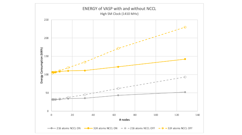
In Figures 1 and 2, the data are normalized to the energy used by one node with NCCL enabled, running at the maximum frequency of 1,410 MHz. All the data shown are for the 216-atom case of hafnia. The vertical axes are matched, so relative energy usage can be seen between NCCL enabled and disabled.

A chart showing energy use relative to default GPU clock of 1,410 MHz as the GPU clock is changed from less than 800 MHz to 1,410. The plots show a smooth curve, and minimum at 1,250 MHz for both NCCL enabled and disabled. NCCL enabled at 128 nodes shows a 60% increase over the baseline, NCCL disabled shows a 200+% increase over the baseline. — *Figure 1. Relative energy use at different GPU clocks (x-axis) for different node counts (separate lines) for NCCL enabled and the 216-atom case*

Chart showing energy use relative to default GPU clock of 1,410 MHz as the GPU clock is changed from less than 800 MHz to 1,410. The plots show a smooth curve, and minimum at 1,250 MHz for both NCCL enabled and disabled. NCCL enabled at 128 nodes shows a 60% increase over the baseline, NCCL disabled shows a 200+% increase over the baseline. — *Figure 2. Relative energy use at different GPU clocks (x-axis) for different node counts (separate lines) for NCCL disabled and the 216-atom case*

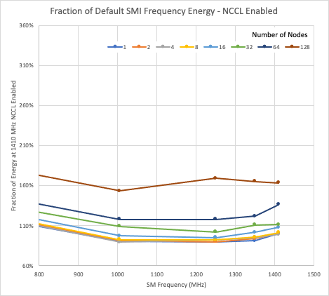
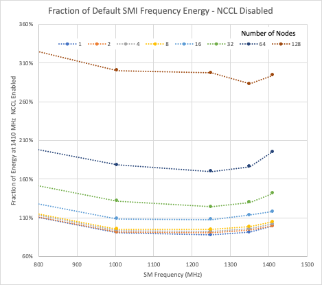
For both the NCCL enabled and disabled cases, reducing the GPU clock offers, at best, a 10% reduction in energy usage compared to the single-node, maximum frequency energy usage. In both cases, the minimum energy usage for most runs is close to the 1,250 MHz GPU clock.

Scalability and energy usage

Our previous investigation showed the significant performance available to NVIDIA GPU users when calculating large atomic systems in VASP within the hybrid DFT level of theory. Though the focus of this work is energy usage and efficiency, performance remains a crucial concern.

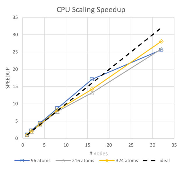
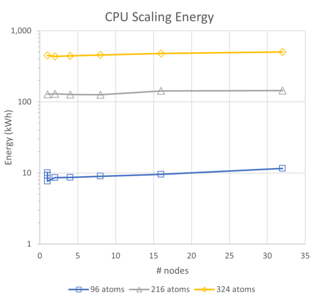
Chart showing the near-linear scaling for the three models: 96, 216, and 423 atoms. — Figure 3. CPU scalability compared to *ideal for 96, 216, and 324 atoms*

Chart showing the energy usage of the three models at about 10 kWh for 96 atoms, 100 for 216 atoms, about 700 kWh for 324 atoms. — *Figure 4. CPU energy usage scaling for 96, 216, and 324 atoms*

To view the energy use trends, we began with a comparison of CPU-only and GPU performance, and energy. Though the CPUs for these systems are two generations behind current state-of-the-art Intel CPUs, they exhibit excellent scalability and a roughly linear trend for energy use. For the range of a single node up to 32 nodes, the energy usage for the 96-atoms case increases by 24%, for 216 atoms it increases by 13%, and for the 324-atom case it increases by 12%.

By comparison, for the GPU runs at the same scales with NCCL enabled, energy increases by 10% at 216 atoms, and 3% at 324 atoms. Though it is not plotted, parallel efficiency for all three CPU-based runs stays above 80%, so the scaling is very good.

In Figures 5 and 6, GPU performance data is shown for the maximum available GPU frequency of 1,410 MHz with NCCL enabled on four A100 GPUs per node. Note that the GPU system is more than an order of magnitude faster than the CPU system, and the scalability (slope of the lines) are essentially parallel, so both are scaling at the same rate.

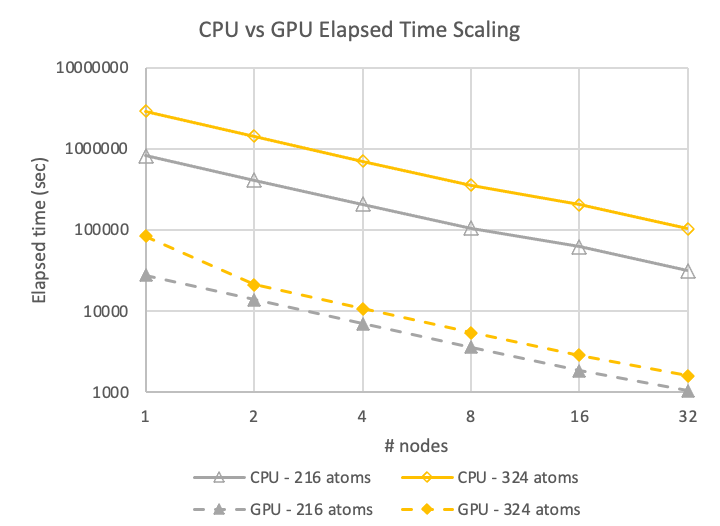
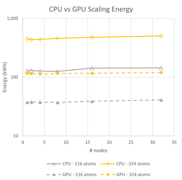
Log-log plot of elapsed time compared to number of nodes, where GPUs are more than an order of magnitude faster than CPUs for both the 216 and 324 atom cases, and both scale roughly linearly — *Figure 5. CPU elapsed time compared to GPU-based systems for 216 and 324 atoms*

A semi-log plot of energy where GPUs use more than a factor of two less energy for both 216 and 324 atom cases. — *Figure 6. CPU energy compared to GPU-based systems for 216 and 324 atoms*

Figure 5 shows that the performance achieved for the 324-atom case on 32 nodes of CPUs is about the same speed as for a single node of A100 GPUs. GPU systems, even though they run at higher power, use less than 20% of the energy compared to CPU-based simulations.

The other item of note is the near invariance in energy use between one and 32 nodes for the GPU system. For the case of hafnia at these sizes, the A100 GPU systems are 5x as energy efficient while delivering more than 32x the throughput in the same elapsed time.

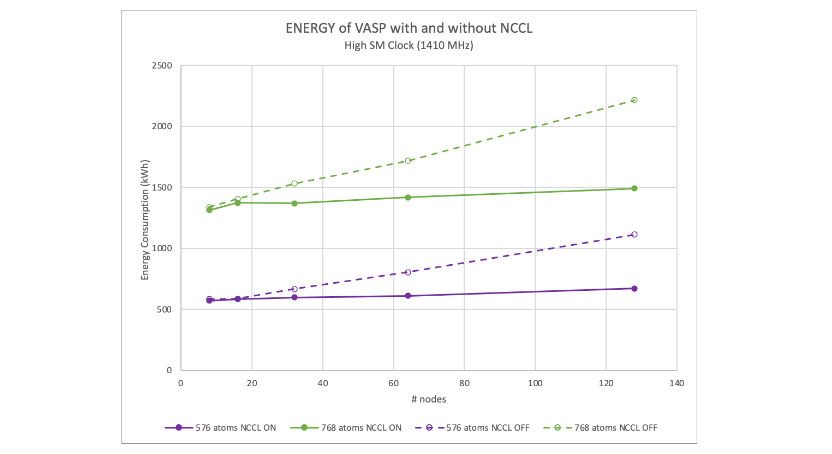
Figures 7 and 8 show the scalability of VASP with NCCL enabled and disabled. NCCL offers about twice the performance at 128 nodes (or 1,024 GPUs). Our previous work showed that the performance for VASP 6.4.0 is slightly better than 6.3.2.

Both figures are plotted relative to the single-node VASP 6.3.2 results. They show a 128-node speedup of 107x compared to 114x for the 576-atom case; and 113x compared to 115x for the 768-atom case.

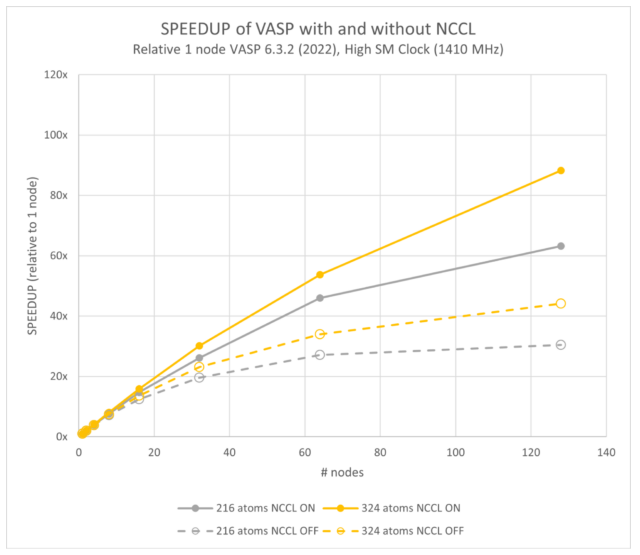
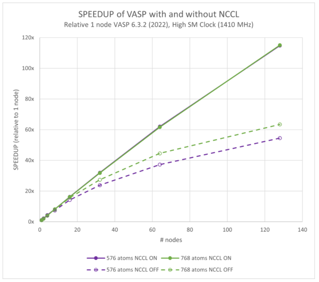
Speedup plot showing good scaling for 216, 324 atom cases up to 64 nodes (1,024 GPUs) and almost a factor of 2 in performance at 64 nodes between NCCL enabled and disabled. — *Figure 7. Strong scaling speedup relative to single-node performance at GPU clock 1,410 MHz for NCCL enabled and disabled and hafnia model sizes for 216 and 324 atoms*

Near-perfect scaling to 128 nodes (2,048 GPUs) for the 576 and 768 atom cases for NCCL enabled, with less scalability for NCCL disabled, and a factor of 2 in performance difference. — *Figure 8. Strong scaling speedup relative to single-node performance at GPU clock 1,410 MHz for NCCL enabled and disabled and hafnia model sizes for 576 and 768 atom*s

The most important effect to note is the performance of the models ranging from 216 atoms to 768. This enables using NCCL instead of only MPI, offering the end user more than 2x the performance for a given number of GPUs. Or similarly, at a given parallel efficiency, an NCCL-enabled VASP hybrid-DFT calculation can be scaled to much higher numbers of GPUs to compress the elapsed time.

Occasionally concerns are expressed that GPU-enabled servers require 4x to 8x the power that a CPU-based server requires. While it is true that GPU servers do require more power, accelerated applications always use far less energy to complete a task compared to a CPU. Energy is power multiplied by time. So, though the GPU server may draw more power (watts) while it is running, it runs for less time and so uses less total energy.

Figure 9 shows a comparison of a GPU and CPU workload, where the CPU workload runs for a long time at low power and the GPU workload finishes much earlier though at a higher power, which enables GPUs to use less energy. The GPU workload runs very quickly at high power. Energy is the area of each of the time histories.

Power compared to time plot showing that GPUs run at high power for short time, CPUs run at low power for a long time. Energy is the area under the curve for each. — *Figure 9. Comparison of a GPU and CPU workload*

Figure 10 shows the energy advantage that using NCCL over MPI-only can provide. Both MPI and NCCL have the GPU server running at roughly the same power level, but because using NCCL scales better, the runtimes are shorter, and thereby less energy is used.

The gap in energy between the two grows with node count simply because the scalability of MPI-only is significantly worse. As the parallel efficiency drops, the simulation runs for a longer time while not doing more productive work, and thereby uses more energy.

Quantitatively, a hafnia hybrid-DFT calculation shows up to 1.8x reduction in energy usage for models between 216 and 768 atoms running at maximum GPU frequency at 128 nodes for using NCCL (Figures 10 and 11).

Using lower numbers of nodes reduces the energy difference because the MPI-only simulations have a relatively higher parallel efficiency when running on fewer nodes. The tradeoff is that the runtime per simulation is extended.

Energy use for 216 and 324 atom cases from one to 128 nodes where NCCL enabled and disabled start at the same energy, and diverge with NCCL disabled using 1.5-2.0x more energy at 128 nodes. — *Figure 10. Energy used at GPU clock 1,410 MHz for NCCL enabled and disabled and hafnia model sizes from 216 atoms and 324 atoms*

Energy use for 576 and 768 atom cases from one to 128 nodes where NCCL enabled / disabled start at the same energy, and diverge with NCCL disabled using 1.5-2.0x more energy at 128 nodes. — *Figure 11. Energy used at GPU clock 1,410 MHz for NCCL enabled and disabled and hafnia model sizes from for 576 and 768 atoms*

As a VASP user or an HPC center manager, you may be asking yourself, “For a given large system of atoms, what is the most efficient point, or how many nodes are needed per simulation?” This is a very good question—one that we expect more and more people will be asking in the near future.

Generally speaking, the fewer the nodes, the closer to 100% parallel efficiency the run will be, and will thereby use less energy. Figure 7 of Scaling VASP with NVIDIA Magnum IO shows the parallel efficiency, and Figures 10 and 11 of this post show the energy.

However, other factors such as researcher time, publishing deadlines, and external influences can increase the value of having simulation results sooner. In these cases, maximizing the number of runs completed in a given time or minimizing the end-to-end wait time for results suggests less energy will be used if the algorithm is configured to obtain the best parallel efficiency. For example, a run with NCCL enabled.

Maximizing application performance against energy usage constraints also helps optimize the return on investment for the HPC center manager.

Balancing speed and energy

Figure 10 or 11 might be interpreted as a recommendation to run a VASP simulation on as few nodes as possible. For HPC centers more focused on maximum efficiency than scientific output, that may be the right decision. We do not anticipate such an attitude to be common.

Doing so, however, could easily ignore costs, which are not captured in a single metric like energy per simulation. For instance, researcher time is arguably the most precious resource in the scientific toolchain. As such, most HPC centers will want to explore a more balanced approach of reducing energy usage while minimizing the performance impact to their users.

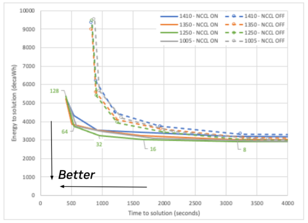
This is a multi-objective optimization problem with a family of solutions depending on the relative weight of the time-to-solution and energy-to-solution objectives. We therefore expect a rigorous analysis to produce a pareto front of optimal solutions.

A quick approach, however, is to plot energy to solution on the vertical axis, and time to solution on the horizontal axis. By visualizing the data this way, the best compromise between these two is the datapoint closest to the origin.

Figure 12 shows the separation between NCCL enabled and NCCL disabled as the cluster of dotted lines and the cluster of solid lines, where the solid lines reach an area much closer to the optimum. It also shows some difference between the maximum performance line (blue) and maximum efficiency line (green) for both NCCL enabled and disabled.

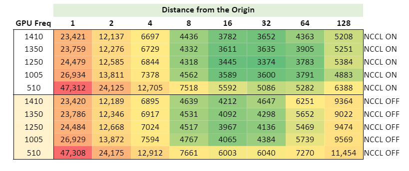
Plot of energy to solution compared to time to solution where lower of both parameters is labeled “better” for NCCL enabled and disabled for four different GPU clocks: 1,410, 1,350, 1,250, 1,005. — *Figure 12. Energy per jobs compared to runtime used on a 216-atom hafnia study*

It is difficult, however, to draw a conclusion about the optimum point to run. Is it 32 or 64 nodes? To help answer this question, Figure 13 shows a heat map calculating the distance to the origin, where green is closest to the optimum.

Red to green heat map of distance from the origin, where the minimum distance represents the best compromise between time to solution and energy to solution. Best are 1,350 MHz and 1,250 MHz frequency, NCCL-enabled, 16, 32 nodes. Worst is NCCL enabled or disabled for one node at 510 MHz. — *Figure 13. Heat map of distance from the origin, where green is closest to the optimum*

Summary

Energy will continue to be a precious commodity for the foreseeable future. We have shown here and in our previous post that the NVIDIA accelerated computing platform of hardware and software is vastly more performant for multi-node simulations using VASP for medium and large-sized molecular hybrid-DFT calculations compared to both a CPU-only platform as well as an accelerated platform that uses MPI only.

Based on these results, we urge researchers using VASP for anything but the smallest systems to do so using the NVIDIA accelerated platform. This approach uses less energy per expended kWh and enables more work per unit of time.

The results of this investigation show that the energy use of simulations varies by more than two orders of magnitude depending on the atom count. However, the optimization opportunity is not as large as the total use.

The energy savings opportunity associated with using NVIDIA Magnum IO NCCL ranges from 41 kWh in the 216-atom case at 128 nodes at best time to solution (1,410 MHz for the A100 GPU) to 724 kWh per simulation for the 768-atom case at 128 nodes. Running for best energy to solution (1,250 MHz) doesn’t change the number materially for 216 atoms, and drops the difference between NCCL enabled and disabled to 709 kWh per simulation for 768 atoms.

In order of most energy savings for minimum impact to runtime, our recommendation for running multi-node, multi-GPU simulations for large VASP systems follows:

Run VASP on the NVIDIA accelerated GPU platform rather than on CPUs only.
Use NVIDIA Magnum IO NCCL to maximize parallel efficiency.
Run a 216-atom hybridDFT calculation between 16 and 64 nodes (128 to 512 A100 GPUs); more for larger systems, and less for smaller.
Run at the MaxQ point of 1,250 MHz (GPU clock) to get the last 5-10% energy savings.

Looking beyond the hybrid DFT in VASP analyzed in this post, software developers can also conserve energy by (in descending order of impact):

Accelerating applications with GPUs
Optimizing as much as possible, including hiding unproductive, but necessary parts
Having users run at optimized frequencies

For more information about NCCL and NVIDIA Magnum IO, watch the GTC sessions, Scaling Deep Learning Training: Fast Inter-GPU Communication with NCCL and Optimizing Energy Efficiency for Applications on NVIDIA GPUs.