Quantum computing aspires to deliver more powerful computation in faster time for problems that cannot currently be addressed with classical computing. NVIDIA recently announced the cuQuantum SDK, a high-performance library for accelerating the development of quantum information science. cuQuantum recently was used to break the world record for the MaxCut quantum algorithm simulation running on the DGX SuperPOD, with 8x more qubits than prior work.
The initial target application for cuQuantum is acceleration of quantum circuit simulations, and it consists of two major libraries:
- cuStateVec: Accelerates state vector simulations.
- cuTensorNet: Accelerates tensor network simulations.
In this post, we provide an overview of both libraries, with a more detailed discussion of cuTensorNet.
Why use cuStateVec?
The cuStateVec library from the cuQuantum SDK provides a high-performance solution for state vector-based simulation through optimized GPU kernels for most use cases that arise in simulators. While the state vector method is great for running deep quantum circuits, simulations of quantum circuits with large numbers of qubits, which grow exponentially, are impossible to run even on today’s largest supercomputers.
Why use cuTensorNet?
As an alternative, the tensor network method is a technique that represents the quantum state of N qubits as a series of tensor contractions. This enables quantum circuit simulators to handle circuits with many qubits by trading space required by the algorithms with computation. Depending on circuit topology and depth, this can also get prohibitively expensive. Then, the main challenge is to compute these tensor contractions efficiently.

The cuTensorNet library from the cuQuantum SDK provides a high-performance solution for these types of tensor network computations.
The cuTensorNet library offers both C and Python APIs to provide access to high-performance tensor network computations for accelerating quantum circuit simulation. The APIs are flexible, enabling you to control, explore, and investigate each of the algorithmic techniques implemented.
cuTensorNet algorithmic description
In this section, we discuss the different algorithms and techniques used in cuTensorNet. It includes two main components: pathfinder and execution.
The pathfinder provides an optimal contraction path with minimal cost in a short elapsed time and the execution step computes that path on the GPU using efficient kernels. These two components are independent of each other and are interoperable with any other external library providing similar functionality.
Pathfinder
At a high level, the approach taken in cuTensorNet is hyper-optimization around a graph partitioning-based pathfinder. For more information, see Hyper-optimized tensor network contraction.
The role of a pathfinder is to find a contraction path that minimizes the cost of contracting the tensor network. Many algorithmic advancements and optimization were developed to make this step fast, and it will become even faster.
Finding an optimal contraction path is strongly dependent on the size of the network. The larger the network, the more techniques and computational effort are needed to find the optimal contraction path.
The cuTensorNet pathfinder consists of three algorithmic modules (Figure 2).

- Simplification: A technique that preprocesses the tensor network to find all sets of obvious straightforward contractions. It removes them from the network and replaces each set by its final tensor. The result is a smaller network that is easier to process in the following modules.
- Path computation: The heart of the pathfinder component. It is based on a graph-partitioning step, followed by a second step that uses a reconfiguration adjustment and slicing technique. The graph partitioning is called recursively to split the network and form a contraction path (for example, a pairwise contraction tree).
- Hyper-optimizer: A loop over the path computation module where at each iteration a contraction path is formed. For each iteration, the hyper-optimizer creates a different configuration of parameters for the path computation while keeping track of the best path found. You change or fix any of these configuration parameters as you like. All configuration parameters can be set by
cutensornetContractionOptimizerConfigSetAttribute. For more information, see the cuTensorNet documentation.
The generated path from the first step might not be close to optimal, so the reconfiguration adjustment is usually performed. Reconfiguration chooses several small subtrees within the overall contraction tree and attempts to improve their contraction cost, decreasing the overall cost if possible.
Another feature of the path computation module is the slicing technique. The primary goal of slicing is to fit the network contraction process into the available device memory. Slicing accomplishes this by excluding certain tensor modes and explicitly unrolling their extents. This generates many similar contraction trees, or slices, where each corresponds to one of the excluded modes.
The contraction path, or tree, does not change. Only some modes are excluded in this case and the computation of each slice is independent from the others. Consequently, slicing can be considered as one of the best techniques to create independent work for different devices.
Practical experience indicates that finding an optimal contraction path can be sensitive to the choice of configuration parameters of each of the techniques used here. To increase the probability of finding the best contraction path, we encapsulate this module inside a hyper-optimizer.
Pathfinding performance
There are two relevant metrics when considering the performance of a pathfinder: the quality of the path found, and the time taken to find that path. The former is plotted in Figure 3, measured by the cost of the resulting contraction in FLOPS. The circuits used for benchmarking are random quantum circuits from Google Quantum AI’s 2019 quantum supremacy paper, at depth 12, 14, and 20.
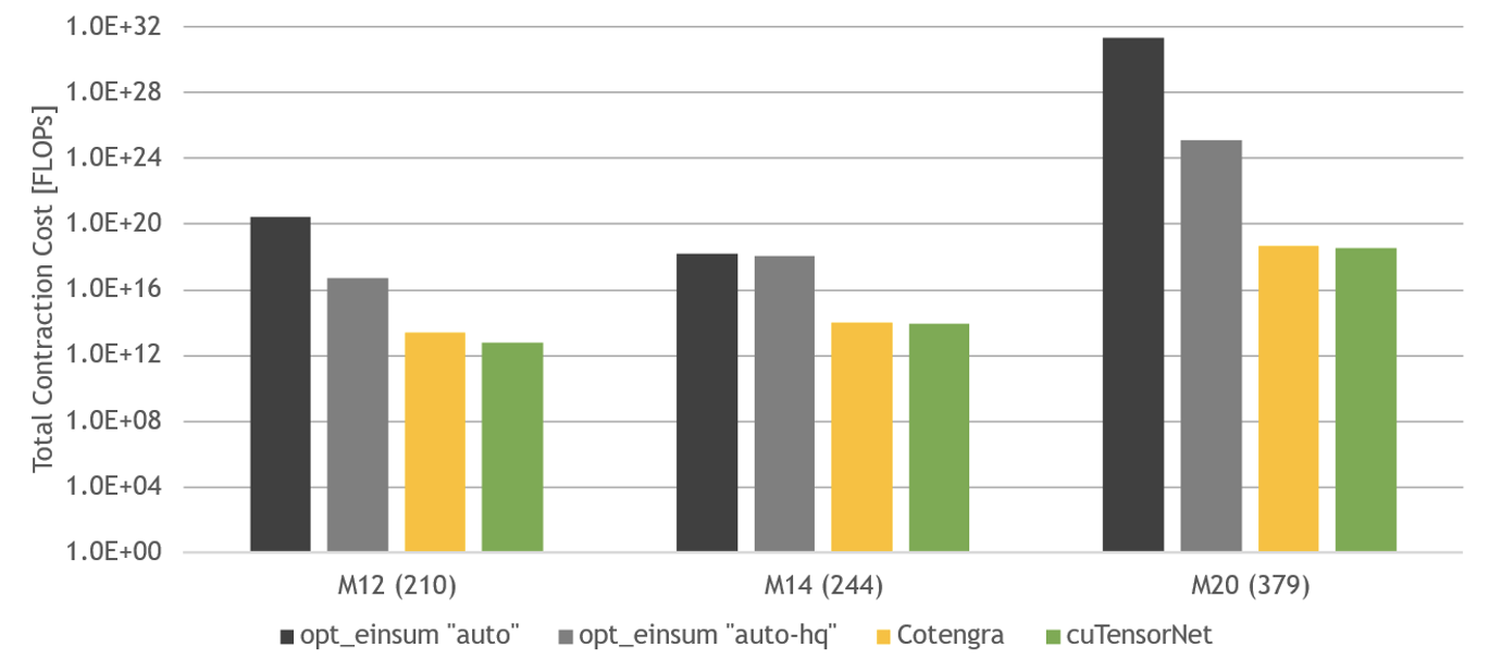
cuTensorNet performs well compared to the opt_einsum library in finding an optimal path, and slightly better than Cotengra for these circuits.
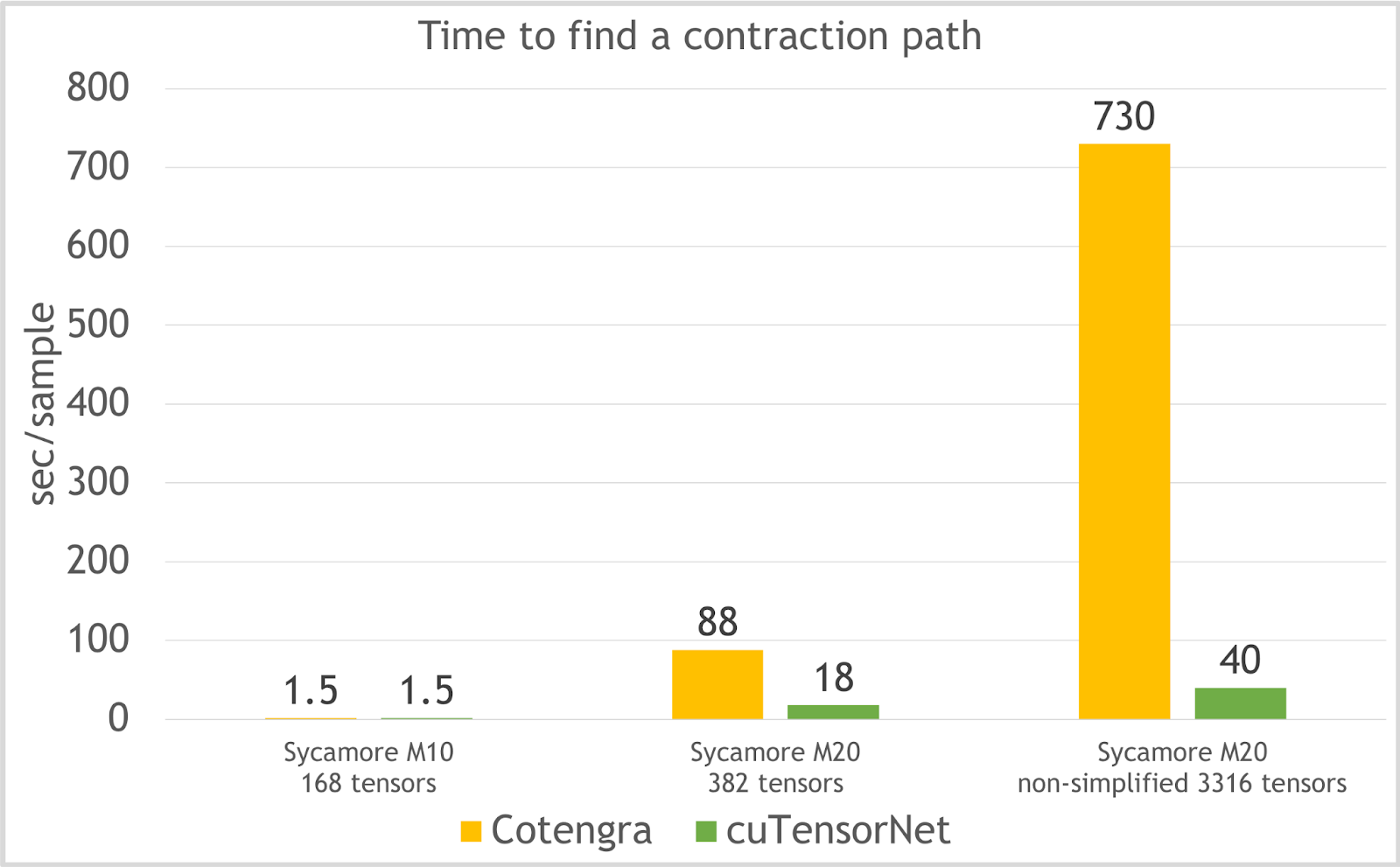
cuTensorNet also finds a high-quality path quickly. The time taken to find a contraction for cuTensorNet compared to Cotengra is plotted in Figure 4, for the Sycamore quantum circuits problems with different depth. For the most complex problem with over 3,000 tensors in the network, cuTensorNet still finds its optimal path in just 40 seconds.
Execution
The execution component relies on the cuTENSOR library as the backend for efficient execution on the GPU. It consists of the following phases:
- Planning: The decision engine of the execution component. It analyzes the contraction path, deciding the best way to execute it on GPU using the minimal workspace. It also decides on the best kernels to be used for each of the pairwise contractions.
- Computation: This phase computes all the pairwise contractions using the cuTENSOR library.
- Autotuning: (Optional) Different kernels based on different heuristics are tried for pairwise contraction and the best is chosen.
Execution performance
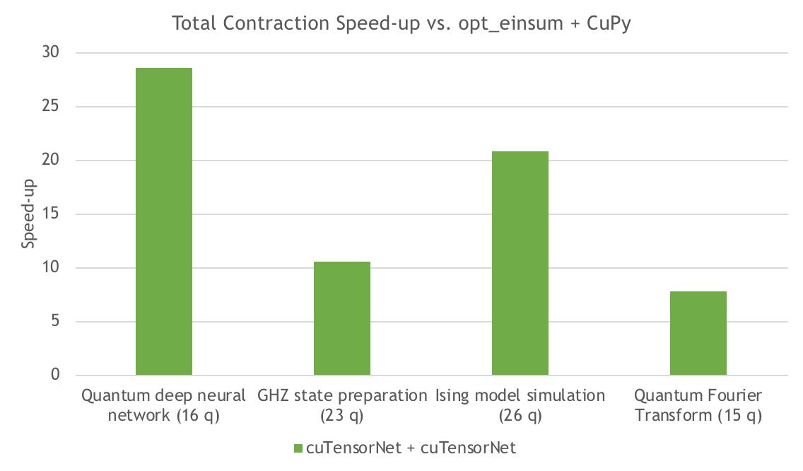
Figure 5 measures the speedup of the contraction execution for cuTensorNet compared to CuPy, for several different circuits. Depending on the circuit, cuTensorNet offers around an 8-20x speedup for the contraction execution.
cuTensorNet example
cuTensorNet provides both C and Python APIs that allow you to compute tensor network contractions efficiently without requiring any expertise on how to find the best contraction path or how to execute it on GPUs.
High-level Python APIs
cuTensorNet offers high-level Python APIs that are interoperable with NumPy and CuPy ndarrays and PyTorch tensors. For example, the einsum expression of a tensor network can be used in a single function call to contract. cuTensorNet performs all the required steps, returning the contracted network as a result.
import cupy as cp
import cuquantum

# Compute D_{m,x,n,y} = A_{m,h,k,n} B_{u,k,h} C_{x,u,y}
# Create an array of extents (shapes) for each tensor
extentA = (96, 64, 64, 96)
extentB = (96, 64, 64)
extentC = (64, 96, 64)
extentD = (96, 64, 96, 64)

# Generate input tensor data directly on GPU
A_d = cp.random.random(extentA, dtype=cp.float32)
B_d = cp.random.random(extentB, dtype=cp.float32)
C_d = cp.random.random(extentC, dtype=cp.float32)

# Set the pathfinder options
options = cuquantum.OptimizerOptions()
options.slicing.disable_slicing = 1  # disable slicing
options.samples = 100                # number of hyper-optimizer samples

# Run the contraction on a CUDA stream
stream = cp.cuda.Stream()
D_d, info = cuquantum.contract(
    'mhkn,ukh,xuy->mxny', A_d, B_d, C_d,
    optimize=options, stream=stream, return_info=True)
stream.synchronize()

# Check the optimizer info
print(f"{info[1].opt_cost/1e9} GFLOPS")
From this code example, you can see that all cuTensorNet operations are encapsulated in the single contract API. The output for this example is 14.495514624 GFLOPS: the number of floating-point operations estimated based on the contraction path found by the path finder. To perform the same steps manually, you can also use the cuQuantum.Network object.
Low-level APIs
As previously discussed, the C and Python APIs are designed in a straightforward expressive fashion. You can call the pathfinder function to get an optimized path, followed by a call to perform the contraction on the GPU using that path.
For advanced users, the cuTensorNet library API is designed to grant access to all algorithmic choices available to enable research in this field. For example, you can control how many hyper-optimizer samples the pathfinder can try to find the best contraction path.
There are dozens of parameters that you can modify or control. These are accessible through the helper functions and allow the simple functionalities API to remain unchanged. You are also allowed to provide your own path. For more information about the lower-level options and examples of how to use them, see cuquantum.Network.
Summary
The cuTensorNet library of the NVIDIA cuQuantum SDK aims to accelerate tensor network computation on GPUs. In this post, we showed the speedup over state-of-the-art tensor network libraries on key quantum algorithms.
There is extensive development to improve cuTensorNet and expand it with new algorithmic advancements as well as multi-node, multi-GPU execution.
The cuTensorNet library goal is to provide a useful tool for groundbreaking developments in quantum computing. Have feedback and suggestions on how we can improve the cuQuantum libraries? Send email to cuquantum-feedback@nvidia.com.
For more information, see the following resources:
- cuQuantum beta (includes cuTensorNet)
- cuQuantum documentation
- NVIDIA/cuQuantum GitHub repo