In the first post, Rendering in Real Time with Spatiotemporal Blue Noise, Part 1, we introduced the time axis and importance sampling to blue noise textures. In this post, we take a deeper look, show a few extensions, and explain some best practices.
For more information, download spatiotemporal blue noise textures and generation code at NVIDIAGameWorks/SpatiotemporalBlueNoiseSDK on GitHub.
How and why does blue noise work?
Neighboring pixels in blue noise textures have very different values from each other, including wrap around neighbors, as if the texture were tiled. The assumption is that when you have a function that renders a pixel \(y=f(x)\), small changes in x result in small changes in y, and that big changes in x result in big changes in y.
When you put very different neighbor values in for x, you also then get very different neighbor values out for y, tending to make the rendered result have blue noise error patterns. This assumption usually holds, unless your pixel rendering function is a hash function, on geometry edges, or on shading discontinuities.
It’s also worth noting that each pixel in spatiotemporal blue noise is a progressive blue noise sequence over time but is progressive from any point in the sequence. This can be seen when looking at the DFT and remembering that the Fourier transform assumes infinite repetition of the sequence being transformed.
There are no seams in the blue noise that would distort the frequency content. This means that when using TAA, where each pixel throws out its history on different timelines, every pixel is immediately on a good, progressive sampling sequence when rejecting history, instead of being on a less good sequence until the sequence restarts, as is common in other sampling strategies. In this way, each pixel in spatiotemporal blue noise is toroidally progressive.
It is worth mentioning is that that pixels under motion under TAA lose temporal benefits and our noise then functions as purely spatial blue noise. Pixels that are still even for a moment gain temporal stability and lower error, however, which is then carried around by TAA when they are in motion again. In these situations, our noise does no worse than spatial blue noise, so should always be used instead, to gain benefits where available and do no worse otherlwise.

Denoising blue noise
Blue noise is more easily removed from an image than white noise due to digital signal processing reasons. White noise has randomization in all frequencies, while blue noise has randomization only in high frequencies.
A blur, such as a box filter or a Gaussian blur, is a low-pass filter, which that means it removes high frequencies but enables low frequencies to remain.
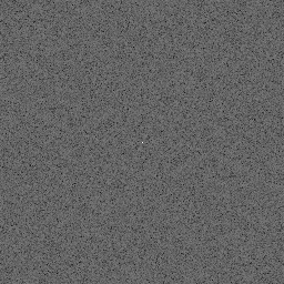
- When white noise is blurred, it turns into noisy blobs, due to lower frequency randomization surviving the low-pass filter.
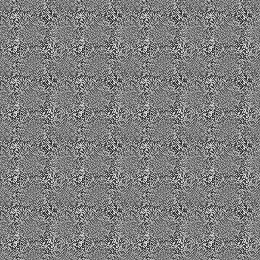
- When blue noise is blurred, the high frequency noise goes away and leaves the lower frequencies of the image intact.
Blue noise uses Gaussian energy functions during its creation so it is optimized to be removed by Gaussian blurs. If you blur blue noise with a Gaussian function and are seeing noisy blobs remain, that means you must use a larger sigma in the blur, due to the lower frequencies of the blue noise passing through the filter. There may be a balance between removing those blobs and preserving more detail in the denoised image. It depends on your preferences.
Figures 2, 3, and 4 show how blue noise compares to white noise both when used raw, as well as when denoised.

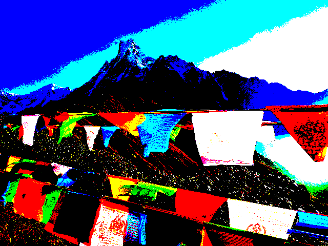
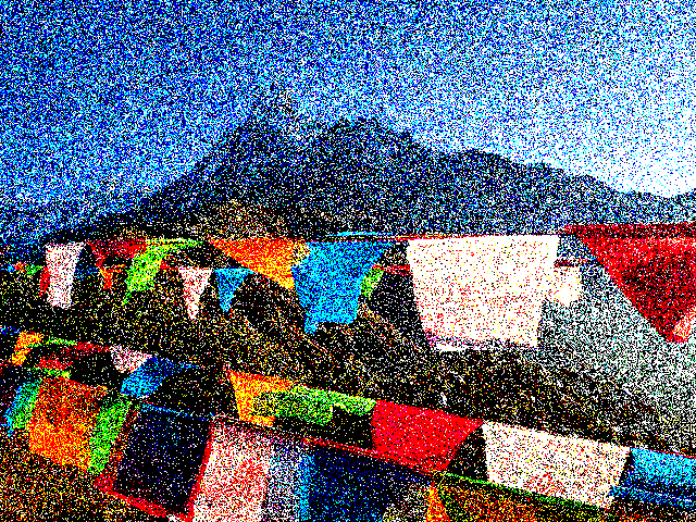
In Figure 3, both images have only eight colors total, as they are only 1-bit per color channel. There are many more recognizable and finer details in the blue-noise–dithered image!
To see the reason why blue noise denoises so much better than white noise, look at them in frequency space. You apply a Gaussian blur through convolution, which is the same as a pixel-wise multiplication in frequency space.
- If you multiply the blue noise frequencies by the Gaussian kernel frequencies, there will be nothing left, and it will be all black; the Gaussian blur removes the blue noise.
- If you multiply the white noise frequencies by the Gaussian kernel frequencies, you end up with something in the shape of the Gaussian kernel frequencies (low frequencies), but they are randomized. These are the blobs left over after blurring white noise.
Figure 5 shows the frequency magnitudes of blue noise, white noise, and a Gaussian blur kernel.

Tiling blue noise
Blue noise tiles well due to not having any larger scale (lower frequency) content. Figure 6 shows how this is true but also shows that blue noise tiling gets more obvious at lower resolutions. This is important because blue noise textures are most commonly tiled across the screen and used in screen space. If you notice tiling when using blue noise, you should try a larger resolution blue noise texture.

Getting more than one value per pixel
There may be times you want more than one spatiotemporal blue noise value per pixel, like when rendering multiple samples per pixel.
One way to do this is to read the texture at some fixed offset. For instance, if you read the first value at (pixelX, pixelY) % textureSize, you might read the second value at (pixelX+5, pixelY+7) % textureSize. This essentially gives you an uncorrelated spatiotemporal blue noise value, just as if you had a second spatiotemporal blue noise texture you were reading from.
The reason this works is because blue noise textures have correlation only over short distances. At long distances, the values are uncorrelated, as shown in Figure 7.
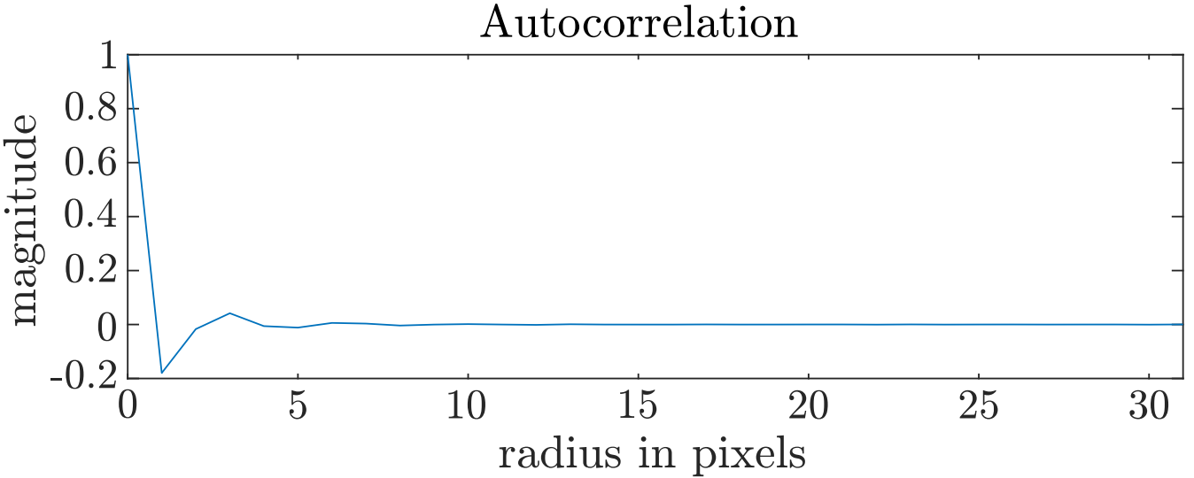
Ideally if you want N spatiotemporal blue noise values, you should read the blue noise texture at N offsets that are maximally spaced from each other. A good way to do this is to have a progressive low-discrepancy sequence into which you plug the random number index, and it gives you an offset at which to read the texture.
We have had great success using Martin Robert’s R2 sequence to plug in an index, get a 2D vector out in [0,1), and multiply by the blue noise texture size to get the offset at which to read.
There is another way to get multiple values per pixel though, by adding a rank 1 lattice to each pixel. When done this way, it’s similar to Cranley-Patterson rotation on the lattice but using blue noise instead of white noise.
- For scalar blue noise, we’ve had good results using the golden ratio or square root of two.
- For non-unit vec2 blue noise, we’ve had good results using Martin Robert’s R2 sequence.
You could in fact use this same method to turn a 2D blue noise texture into spatiotemporal blue noise but would lose some quality in the process. For more information, see the SIGGRAPH 2021 paper that talks about this method, Lessons Learned and Improvements when Building Screen-Space Samplers with Blue-Noise Error Distribution.
This method sometimes converges better than spatiotemporal blue noise but has a more erratic error graph, making it less temporally stable, and damages the blue noise frequency spectrum. Figure 8 shows the frequency damage and Figure 8 shows some convergence behavior. For more information about convergence characteristics, see the simple function convergence section later in this post.
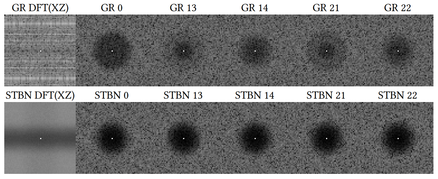
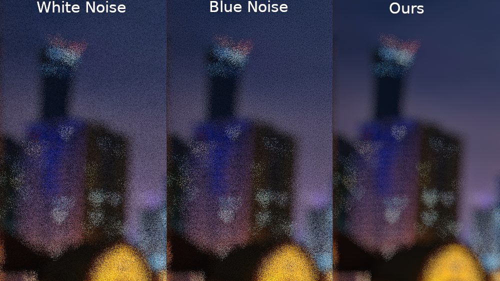
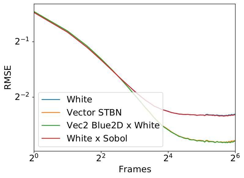
Figure 9 shows a graph comparing real vector spatiotemporal blue noise to the R2 low discrepancy sequence that uses a single vector blue noise texture for Cransley-Patterson rotation.
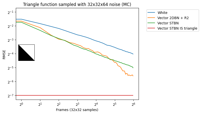
These two methods are the way that others have animated blue noise previously. Either the blue noise texture is offset each frame, which makes it blue noise over space and white noise over time, or a low-discrepancy sequence is seeded with blue noise values, making it be damaged blue noise over space, but a good converging sequence over time.
Making vector-valued spatiotemporal blue noise through curve inversion
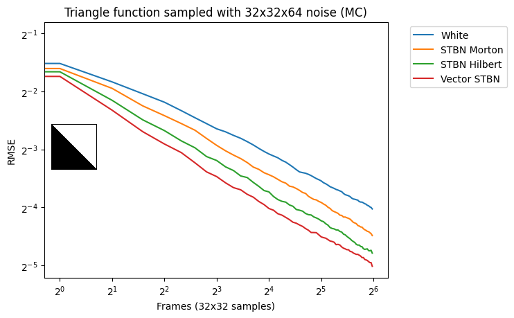
If you have a scalar spatiotemporal blue noise texture, you can put it through an inverted Morton or Hilbert curve to make it into a vector-valued spatiotemporal blue noise texture. We’ve had better results with Hilbert curves. While these textures don’t perform as well as the other methods of making spatiotemporal blue noise, it is much faster and can even be done in real time (Figure 10).
An interesting thing about this method is that we’ve found it works well with all sorts of dither masks or other scalar-valued (grayscale) noise patterns: Bayer matrices, Interleaved Gradient Noise, and even stylized noise patterns.
In all these cases, you get vectors that, when used in rendering, result in error patterns that take the properties and looks of the source texture. This can be fun for stylized noise rendering, but also means that in the future, if other scalar sampling masks are discovered, this method can likely be used to turn them into vector-valued masks with the same properties.
Stratification
The energy function of vector valued spatiotemporal blue noise can be modified to return nonzero only if the following conditions are true:
- The pixels are from the same slice (same z value)
- The temporal histograms of the pixels involved in the swap don’t get worse
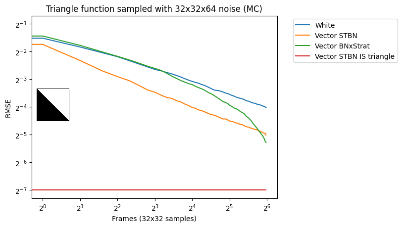
If you do this, you end up with noise that is blue over space but stratified over time; the stratification order is randomized. Because stratification isn’t progressive, it doesn’t converge well until all samples have been taken but does well at that point (Figure 11).
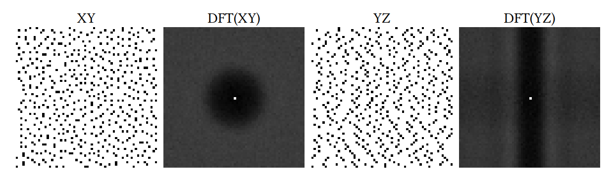
Higher dimensional blue noise
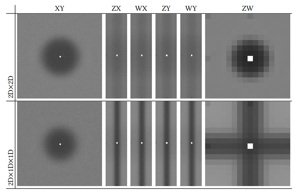
The algorithms for generating spatiotemporal blue noise aren’t limited to working in 3D. The algorithms can be trivially modified to make higher dimensional blue noise of various kinds, although so far, we haven’t been able to find usage cases for them. If spatiotemporal blue noise is 2Dx1D because it is 2D blue noise on XY and 1D blue noise on Z, Figure 12 shows the frequency magnitudes of 4D blue noise, which are 2Dx2D and 2Dx1Dx1D, respectively, with dimensions of 64x64x16x16.
Point sets
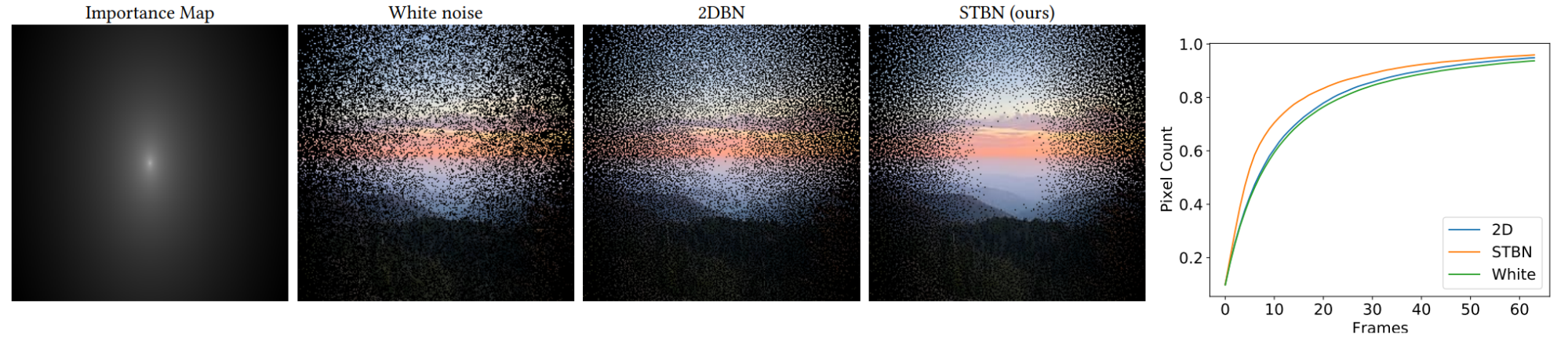
Blue noise textures made with the void and cluster algorithm can be thresholded to a percentage value. That many pixels survive the thresholding and they are blue-noise–distributed. Our scalar-valued spatiotemporal blue noise textures have the same property and result in spatiotemporal blue noise point sets. Figure 13 shows that with the thresholded points of a scalar spatiotemporal blue noise texture, as well as the frequency amplitudes of those thresholded points.
These point sets are such that the pixels each frame are distributed in a pleasing spatial blue noise way, but you also get a different set of points each frame. That means that you get more unique pixels over time compared to white noise or other animated blue noise methods. Figure 14 shows five frames of accumulated samples of an image, using the importance map as the per pixel blue noise threshold value. Our noise samples the most unique pixels the fastest, while also giving a nice blue noise pattern spatially.
Simple function convergence
In this section, we discuss the convergence of simple functions using common types of noise, under both Monte Carlo integration and exponential moving average to simulate TAA.
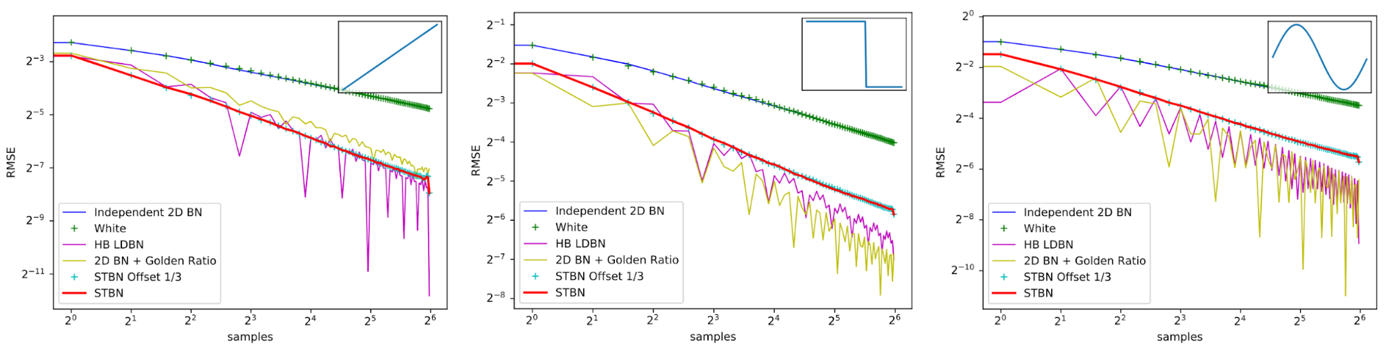
Scalar Monte Carlo integration
Figure 15 shows convergence rates under Monte Carlo integration, like what you would do when taking multiple samples per pixel. HB LDBN is from A Low-Discrepancy Sampler that Distributes Monte Carlo Errors as a Blue Noise in Screen Space. While low-discrepancy sequences can do better than STBN, it is more temporally stable and also makes perceptually good error by being blue noise spatially. STBN Offset 1/3 shows that if you start STBN from an arbitrary place in the sequence, that it still retains good convergence properties. This shows that STBN is toroidally progressive.
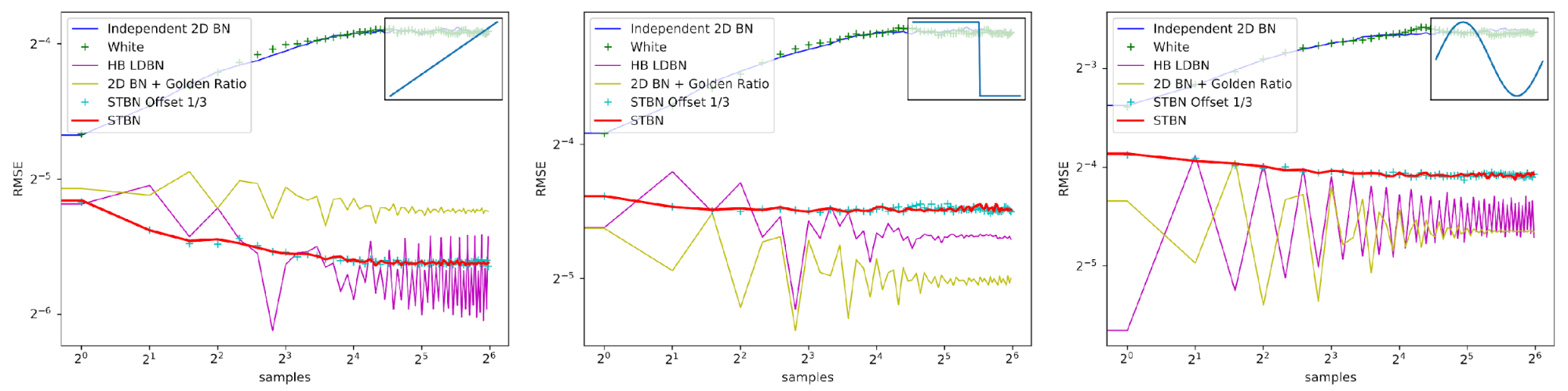
Scalar exponential moving average
Figure 16 shows convergence rates under exponential moving average. Exponential moving average linearly interpolates from the previous value to the next by a value of 0.1. This simulates TAA without reprojection or neighborhood sampling rejection.
Vec2 Monte Carlo integration
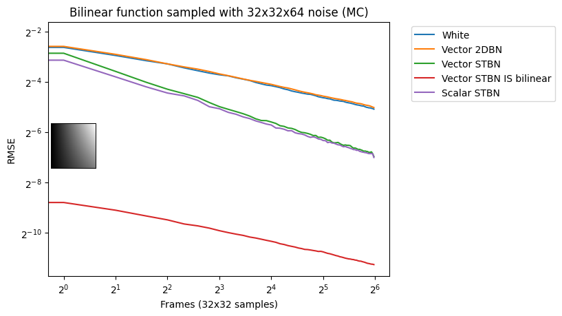
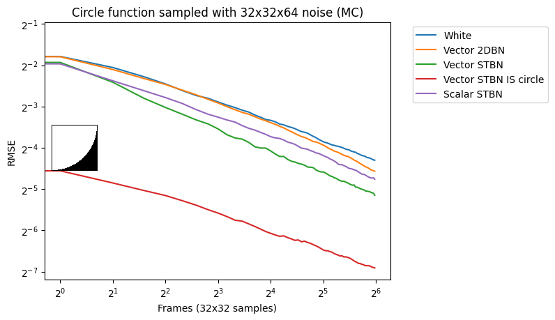
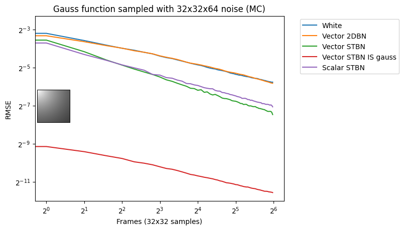
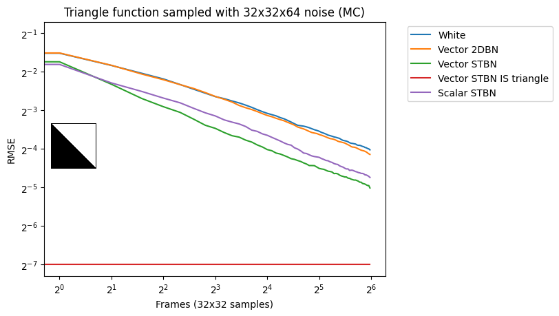
Figure 17 shows convergence rates under Monte Carlo integration. Scalar STBN uses the R2 texture offset method to read two scalar values for this 2D integration. Because of that, it outperforms Vector STBN in the step function, which is ultimately a 1D problem, and also in bilinear, which is ultimately an axis-aligned problem. The reason why importance sampling has any error at all is due to discretization of both the vectors and the PDF values.

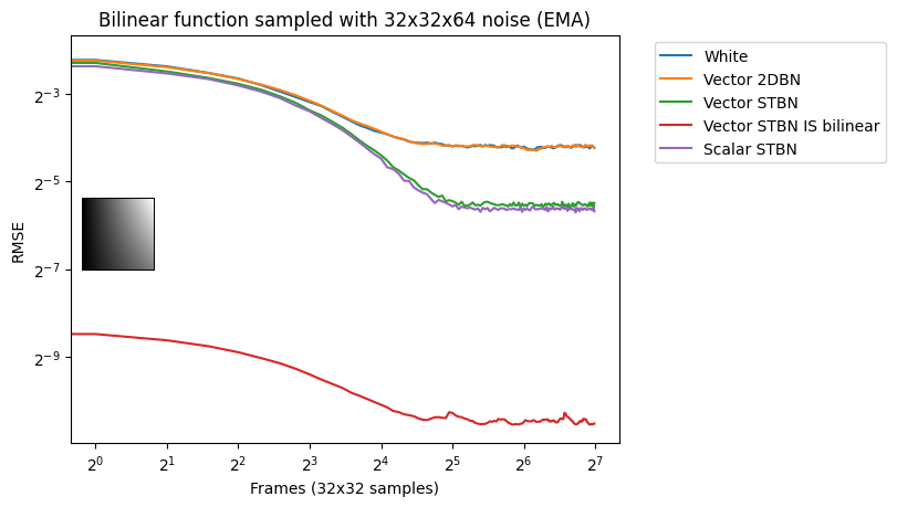
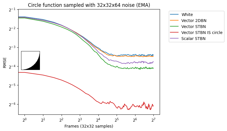
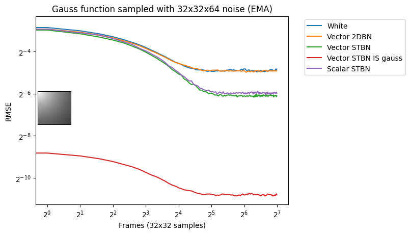
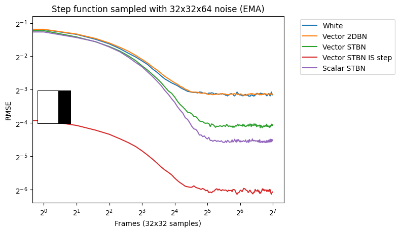
Vec2 exponential moving average
Figure 18 shows convergence under EMA. Exponential moving average linearly interpolates from the previous value to the next by a value of 0.1. This simulates TAA without reprojection or neighborhood sampling rejection.

Conclusion
While blue noise sample points have seen advancements in recent years, blue noise textures seem to have been largely ignored for decades. As shown here, spatiotemporal blue noise textures have several desirable properties for real-time rendering where only low sample counts can be afforded: good spatial error patterns, better temporal stability, and convergence, and toroidal progressiveness, just to name a few.
We believe that these textures are just the beginning, as several other possibilities exist for improvements to sampling textures, whether they are blue-noise–based, hybrids, or something else entirely.
It is worth noting that there are other ways to get great results at the lowest of sample counts, though. For instance, NVIDIA RTXDI is meant for this situation as well but uses a different approach.