
In the high-frequency trading world, thousands of market participants interact daily. In fact, high-frequency trading accounts for more than half of the US equity trading volume, according to the paper High-Frequency Trading Synchronizes Prices in Financial Markets.
Market makers are the big players on the sell side who provide liquidity in the market. Speculators are on the buy side, running experiments and researching processes they expect to profit from. End users are the retail investors who consult retail brokers for advice and transactions. Overall, financial firms are interested in evaluating financial machine learning (ML) algorithms to discover which algorithms are most profitable.
Researchers have published many versions of this type of algorithm recently. We sought to leverage high-frequency data and the explainability of random forest (RF) models, and chose the RF method presented in the paper Investigating Limit Order Book Characteristics for Short-Term Price Prediction: a Machine Learning Approach.
Our study found that hardware acceleration using GPUs reduces the time required for financial ML researchers to obtain prediction results. As most of the runtime can be spent in classifier training, there is, of course, interest in more efficient training methods.
This post walks through our study, including the generated dataset, using limit order book (LOB) data for price prediction, and recommended steps for ML training. We explain how the studied GPU configurations lead to significantly faster ML training time, enabling more efficient and extensive model development.
Dataset
This study used a time series dataset showing real-time stock prices to better understand LOB structure and direction prediction. Provided by market data company Intrinio, the dataset for this study contains samples of actual market prices for NYSE and NASDAQ tickers from the DOW 30 stocks on a 1-second basis.
The 1-second quotes were used as input to ABIDES (Agent-Based Interactive Discrete Event Simulation) to generate LOB data that looks like the LOB of the market. The timestamp on every record is at the second mark; for example: 2019-01-02T14:09:18Z for January 2, the first trading day in 2019.
The CSV file input to ABIDES consists of this column as the first, followed by 30 columns for the prices in US dollars (to two digits) for the DOW 30. This post focuses on the AAPL ticker as a test case.
Synthetic data generation using ABIDES
ABIDES is an approach to simulating the operation of financial markets. It is explained in the recent paper, ABIDES: Towards High-Fidelity Multi-Agent Market Simulation, by researchers at the Georgia Institute of Technology, the University of Georgia, and J.P. Morgan Chase Bank.
ABIDES simulates many individual trading agents who buy and sell assets through exchange agents. Every trade and other event in the simulation is recorded and tied to the agent that performed it. This enables market researchers to analyze in detail how different agent strategies and events affect the simulated market. Importantly, the LOB of a given exchange can be reconstructed after the simulation.
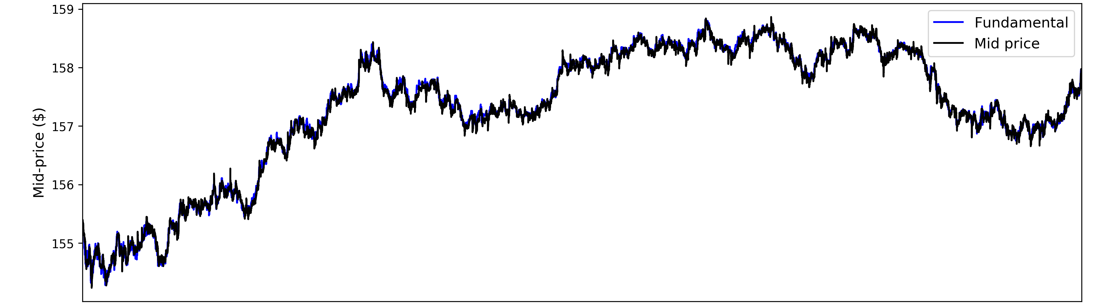
Some agents in an ABIDES simulation base their valuation of an asset on a time series representing the true value of the asset that the agents observe at some frequency with some added noise. This time series is called the fundamental value of the stock. To simulate a more realistic market at a macro scale, we use real historical data for our fundamental value.
To create plausible LOB data for training our RF model, we use 1-second quotes provided by Intrinio as the historical fundamental value for an ABIDES simulation. Figure 1 compares the mid-price of the output LOB data with the 1-second quotes used as the historical fundamental for AAPL.
The LOB as a predictor of short-term price movements
On the bid side of a trade transaction, the buyer would like to pay as little as possible to buy a given security. On the ask side, the seller would like to sell the security for as much as possible. Limit orders are a way of setting these limits on the bid and ask side.
The LOB for a given security is a list of order sizes with security prices on the x-axis and total volume at that price on the y-axis for the bid and ask sides. For example, a buyer is willing to buy 100 shares of the GOOG security at $580 each, so there must be enough shares from those selling to fulfill those 100 shares. See Figure 2 for an example LOB.
The LOB is separated into the bid portion (on the left of the red line in Figure 2), where prices are lower than the mid-market, and the ask portion (on the right of the red line in Figure 2) where prices are higher.
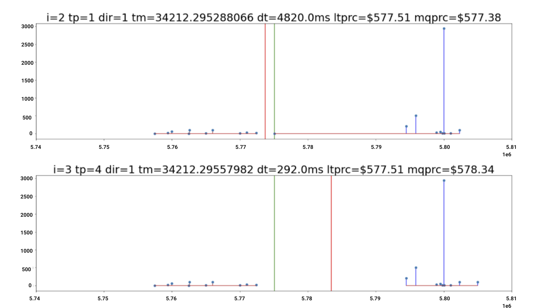
Put simply, buying parties expect to pay lower prices and selling parties expect to gain higher prices in the market. The time points have nine digits behind the decimal point, which reflects the nanosecond accuracy of modern securities exchanges.
Figure 3 shows that accuracy in predicting the immediate direction of price movement increases when more LOB depth is provided to a classifier. This makes intuitive sense, as a classifier has more available information on both sides of the market (bid levels and ask levels) during training.
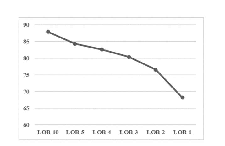
Image credit: Faisal I Qureshi
Accelerate random forest training with RAPIDS
We trained a random forest model to predict short-term price movements with LOB data as input. We trained a classifier to predict whether a given stock price will move upwards, downwards, or stay flat.
Specifically, the goal is to predict whether the average of the next 20 mid-prices (mnext) will be smaller or larger than the average of the previous 20 mid-prices (mprev) by a certain margin. We defined this margin as 0.5 cents, the smallest non-zero difference in mid-prices between any two LOB frames in our dataset.
Our dataset consisted of 90 days of ABIDES-generated data, providing about 7.5 million labeled LOB frames. We used 66% of this dataset as our training set and held out the remaining 33% as a testing set, as in the paper. Our input to the RF model consisted of 40 features, which were the bid and ask prices and volumes at 10 LOB levels.
A label of 2 indicates an upward price movement (mnext – mprev > 0.5 cents), a label of 1 indicates a neutral price movement, and a label of 0 indicates a downward price movement (mnext – mprev < -0.5 cents).
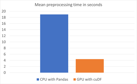
The following experiments were run on one NVIDIA A100 80 GB SXM for RAPIDS cuDF and RAPIDS cuML, and on two AMD EPYC 7742 64-core processors for scikit-learn and pandas. Mid-prices, averages, and labels are computed using both the RAPIDS cuDF library and pandas.
Figure 4 presents a comparison of runtimes. The mean preprocessing time is calculated from 10 runs with 10 warmups for each configuration. This is a labeling step prior to the ML training run shown in Figure 5.
We trained a random forest classifier of 100 trees using both scikit-learn and RAPIDS cuML, and compared training time with each. RAPIDS cuML is a freely available, drop-in replacement for scikit-learn, which enables many popular ML algorithms to be accelerated on the GPU.
Figure 5 shows a comparison of the runtime of the training workload on one NVIDIA A100 80 GB with RAPIDS cuML, and on two AMD EPYC 7742 64-core processors with scikit-learn. Training on CPU is multithreaded with 128 threads, using the scikit-learn n_jobs parameter.
Time is averaged over 50 runs with five warmups, and scikit-learn time is averaged over 10 runs with five warmups. Using the GPU is about 10x faster for training. These results are in line with the 2022 GPU study detailed in Accelerating Machine Learning Training Time for Limit Order Book Prediction.
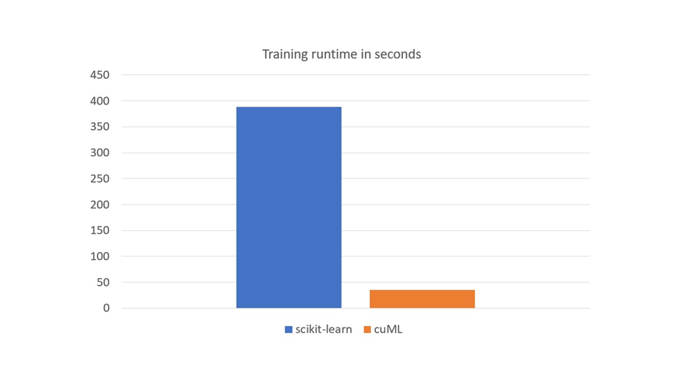
Training on GPU offers more than a 10x speedup for this workload. The iterative nature of ML classifier development makes it time intensive, especially considering the large amount of time series data used in financial markets. In short, the GPU is a game changer in ML algorithms research.
Rising compute needs for financial datasets
While the preceding example uses a single ticker, these high-frequency trading and limit order book use cases need multiple AI systems running the algorithms—equivalent to multiple NVIDIA DGX SuperPODs. Typically, organizations specializing in such use cases require multiple asset classes and trackers.
Hence, the analysis and application of such algorithms can be easily parallelized with cases extending to multiple AI systems needing speedup time and significant compute. For example, quantitative finance, machine learning (such as RAPIDS cuML), and deep learning applications (such as neural nets on top of LOB datasets).
To speed up training when developing financial ML algorithms, you can leverage GPU acceleration by using the RAPIDS suite of libraries:
- RAPIDS cuDF replaces the pandas Python library
- RAPIDS cuML replaces the scikit-learn Python library
Download and install RAPIDS to get started enabling GPUs for your data science workloads. Remember to install an NVIDIA driver and CUDA toolkit beforehand.
