Data Scientists and Machine Learning Engineers often face the dilemma of “machine learning compared to deep learning” classifier usage for their business problems. Depending upon the nature of the dataset, some data scientists prefer classical machine-learning approaches. Others apply the latest deep learning models, while still others pursue an “ensemble” model hoping to get the best of both worlds – explainability and performance.
Machine learning, especially decision trees, and leading up to the more advanced XGBoost models, was maturing earlier than deep learning and has some well-established methods. Deep learning excels in the non-tabular computer vision, language, and speech recognition domains. Whichever you pick, GPUs are accelerating data science use cases to the point where any data analysis on large datasets simply requires them for every day convenience, rapid iteration, and results.

RAPIDS makes leveraging GPUs easier for data scientists through interfaces similar to favorites like scikit-learn and pandas. Here, we are working with a tabular dataset. The classic extract-transform-load process (ETL), is a core-starting point in any data science project.
For GPU-accelerated use cases, the NVIDIA MERLIN application framework for deep recommender systems uses NVTabular – an accelerated feature engineering, preprocessing, and data loading library, which can also be used in other domains such as financial services.
In this article, we demonstrate how to examine competing models, known as challenger models, and use GPU-acceleration to succeed with easy, cost effective, and understandable application of model explainability. When GPU-acceleration is utilized many times during model development, the modeler’s time is used much more effectively by amortizing the training time and cost reductions over dozens of model iterations.
We do this in the context of predicting mortgage delinquencies using the public Fannie Mae mortgage dataset. We also show the simple speedups obtained by an NVTabular data loader for model training. This same example could be extended to credit underwriting, credit card delinquency, or a host of other important class-imbalance binary classification problems.
A common theme in all financial credit risk modeling is the concern for the expected loss. Whether the transaction is a trading agreement between two counter parties where one party owes the other party some amount, or is a loan agreement with borrower owes the lender monthly repayment amounts, we can look at the expected loss, EL, in the following way:
EL = PD x LGD x EAD
Where:
- PD: the probability of default, taking into account all loans in the population
- LGD: the loss given default; a value between 0 and 1, which measures the percentage of unpaid loan
- EAD: the exposure at default, which is the outstanding balance remaining
The PD and EL are attached to a time period, which often can be set to annually or monthly depending on the choice of the firm issuing the loan.
In our case here, the goal is to predict specific individual loans which are most likely to become delinquent, based on their characteristics or features. Thus, we are mostly concentrating on the loans that affect the PD rate, that is, separating those with an expected loss from those with no expected loss.
Machine Learning and Deep Learning approaches
Machine learning (ML) and deep learning (DL) have evolved into cooperative and competing approaches for analytical prediction. It is becoming best practice to consider both approaches and weigh the outcomes of each individual model, or employ ensemble multiple methods to get the best of both worlds for a given application. Either method can extract deep, complex insights out of data to help make decisions.
In many cases, using more advanced ML models delivers real business value over traditional regression models. However, explaining what drove a particular decision with a more advanced model can be difficult, time consuming, and expensive using traditional infrastructure. The model run time is equally important as well as the run time of the explanation steps for interpreting predictions.
In order to be confident in the results, we want to address the new demand for explainability. Existing techniques can be slow, are computationally expensive, and are ideal candidates for GPU acceleration. By moving to GPU accelerated modeling and explainability, teams can improve the processing, accuracy, explainability, and provide results when the business wants them.
Predicting risk in mortgage loans
Default risk can affect us personally when viewed from the consumer side or affect the issuer side as well. Today, in many countries, there are a number of loans being issued for infrastructure improvement projects. One large highway bridge, for example, can require over a billion U.S. Dollars of debt funding. Obviously, financing huge billion dollar projects come with default risk.
Measuring the probability of default is important as the citizens of the governing body certainly do not want to see a default on that issuance. A paper by the Bank of England entitled Machine learning explainability in finance: an application to default risk analysis served as inspiration for the current body of work, which focuses on housing mortgage loans.
The benefits of having this explanation transparency are easy to see in the Bank of England paper. The authors call their approach Quantitative Input Influence (QII) and QII is used for linear logistic and gradient boosted tree machine-learning prediction models. The question arises: what factors contribute most to the defaults?
The authors illustrate the intuitive power of the explanations. They also make observations, which financial modeling practitioners should take note of. The paper demonstrates the ability to engineer adequate accuracy, precision, and recall for default prediction with their precision-recall curve results.
Model explainability may be an important component of discussions with thought leaders, management, external auditors, and regulators. The Shapley values are computed using open source code where the data set consists of six million loans in the U.K. with an approximate 2.5% default rate.
As described in the recent article by NVIDIA authors, default risk is a very common debt use case in the capital markets, banking, and insurance. For example, credit derivatives are a way to speculate on the likelihood of default by tranche and closer to home. Mortgage lenders are deeply interested in whether they will be paid back in a timely fashion.
Ultimately, insurance contracts are ways to cover the risks associated with flooding, theft, or death from the customer viewpoint. From the lender or insurance underwriting viewpoint, predicting these events is critical to the profitability of their business. With the well-known U.S. Fannie Mae public mortgage loan dataset, we are able to examine approaches to risk and the out-of-sample precision, recall, using GPU accelerated training of ML and DL models.
Please see the original article introducing the GPU-accelerated explainability for credit risk and the extension for Shap value clustering and see also this related article for additional interesting explainability and acceleration results for simulating equity instruments.
For this article here, the focus is on the nuances of the ML and DL models and the approaches for explainability. Upon a 90-days past due loan event, concern is raised in the minds of the lending company. The probability of default is of concern due to the replacement costs. A key result of this article is the reported 29-fold speedup in computing Shap values when GPU-acceleration is applied with an algorithm as outlined in this GPUTreeShap paper.
Our Python program predicting defaults for the U.S. Fannie Mae mortgage dataset will use the GPU-accelerated framework known as RAPIDS. RAPIDS provides an application program interface (API) similar to Python pandas for DataFrame operations. The mortgage loan dataset provided in this handy RAPIDS Mortgage Data link has almost two decades of loan performance data with the actual interest rates and borrower characteristics and lender names on record. We have a classic imbalanced class prediction problem with our mortgage loan tabular dataset since only about 4% of all loans are delinquent.
Factorizing for categorical columns
Factors are an important concept in programming languages. Those readers who are familiar with the R language for statistical computing know about factors, created with the factor() function, as a way to categorize columns into a discrete set of values. R, in fact, defaults to factorizing columns, which can be factorized upon input so much so that the user often should override the read.csv() option with the wordy parameter stringsAsFactors=FALSE. Python users will be happy to know that the Python pandas and RAPIDS packages include a very similar factorize() method as mentioned in this article. For our mortgage dataset, zip codes are a classic column to factorize.
df['Zip'], Zip = df['Zip'].factorize()
A series of these transformational statements is an alternative for one-hot encoded columns, reducing the sparsity and memory required in the transformed data. The advantage of factorizing as opposed to using one-hot encodings is that the data frame does not need to grow wider as the number of column values increases yet we still have the advantages of categorical column variables.
XGBoost classifier tuning
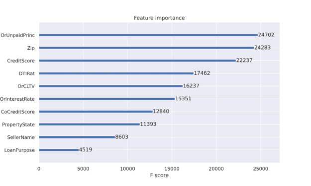
When using decision trees, one obtains the benefit of feature importance. Feature importance is reported to help explain the features used most to make decisions. A feature importance report such as Figure 1 is one of the artifacts that propelled decision trees into a popular classification approach. Decision tree nodes correspond to a set of training dataset rows. Initially we begin with a single node to represent all training rows. Node purity refers to the dataset rows being similar. Node impurity is much more common when we start the process for decision tree training and purity becomes more common as we expand the tree while scanning the dataset. Feature importance is listed in decreasing node impurity, weighted by the chance of reaching that node. The most effective nodes are those that cause the best reduction in impurity and also represent the largest number of samples in the data population.
With decision trees such as the XGBoost classifier, as the decision tree gets expanded through splits from the initial single node to hundreds of nodes, node impurity is not desired when a split occurs to gain accuracy. We will discuss more about explainability soon.
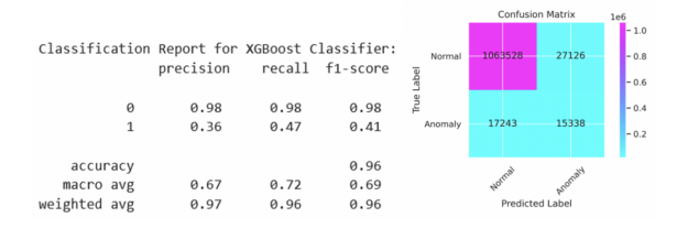
An XGBoost classifier was tuned as part of a Python Jupyter notebook to examine the predictability of loan delinquencies. The inspiration for this work was the article by DeGrave. We focused on the XGBoost classifier in the earlier article and are able to report an improvement in the precision and recall here with factorization. Given a dataset with stimulus variables and the Default output variable, there is a limit to the predictability in the rows of data. Our results in Figure 2 are from a run of 11.2 million individual mortgages from 2007 to 2012 with a subset of 1.1 million loans residing in the test set. Using a customized threshold on the emitted probability of default helped to balance the precision and recall more evenly than using the standard value of 0.5. We show the code sequence below with our best parameters. The code for the XGBoost and PyTorch classifiers explanations is available at https://github.com/NVIDIA/fsi-samples/tree/main/credit_default_risk along with instructions on how to download the mortgage loan dataset.
 params = {
       'num_rounds':     100,
       'max_depth':      12,
       'max_leaves':     0,
       'alpha':          3,
       'lambda':         1,
       'eta':            0.17,
       'subsample':      1,
       'sampling_method':   'gradient_based',
       'scale_pos_weight': scaling, # num_negative_samples/num_positive_samples
       'max_delta_step': 1,
       'max_bin':        2048,
       'tree_method':    'gpu_hist',
       'grow_policy':    'lossguide',
       'n_gpus':         1,
       'objective':      'binary:logistic',
       'eval_metric':    'aucpr',
       'predictor':      'gpu_predictor',
       'num_parallel_tree': 1,
       "min_child_weight":  2,
       'verbose':        True
 }

 if use_cpu:
       print('training XGBoost model on cpu')
       params['tree_method'] = 'hist'
       params['sampling_method'] = 'uniform'
       params['predictor'] = 'cpu_predictor'

 dtrain = xgb.DMatrix(X_train, label=y_train)
 dtest = xgb.DMatrix(X_test, label=y_test)

 evals = [(dtest, 'test'), (dtrain, 'train')]

 model = xgb.train(params, dtrain, params['num_rounds'], evals=evals,
                         early_stopping_rounds=10)
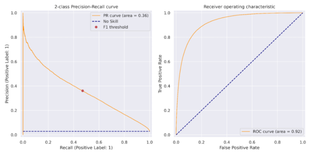
We can see preceding that the objective for the XGBoost training step is binary:logistic and the evaluation metric is the area-under-curve for precision and recall, known as aucpr. After the model was trained, the threshold corresponding to the maximum F1 score was calculated on the training set. This threshold was applied to the predictions on the test set with the results shown in Figure 2 and is indicated as the red dot in the precision-recall curve in Figure 3.
Speed up PyTorch Deep Learning training with NVTabular
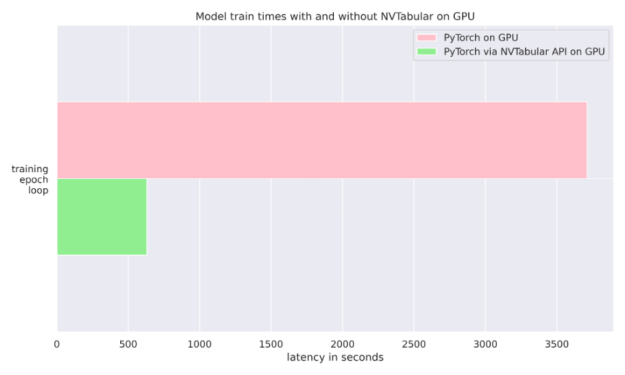
The NVIDIA NVTabular Python package is a feature engineering and preprocessing library for tabular data that is designed to quickly and easily manipulate terabyte scale datasets and train deep learning (DL) based recommender systems. It can be installed using Anaconda or Docker or using pip with the nvtabular keyword. In our case, we simply use it to feed data into our PyTorch classifier during training. We also compared the run-time of using a plain PyTorch Dataloader compared to NVTabular’s Asynchronous PyTorch Dataloader. We found for our mortgage dataset that NVTabular delivers a 6-fold advantage over not using it where both runs were completed on the same GPU. See Figure 4 and this article for more details.
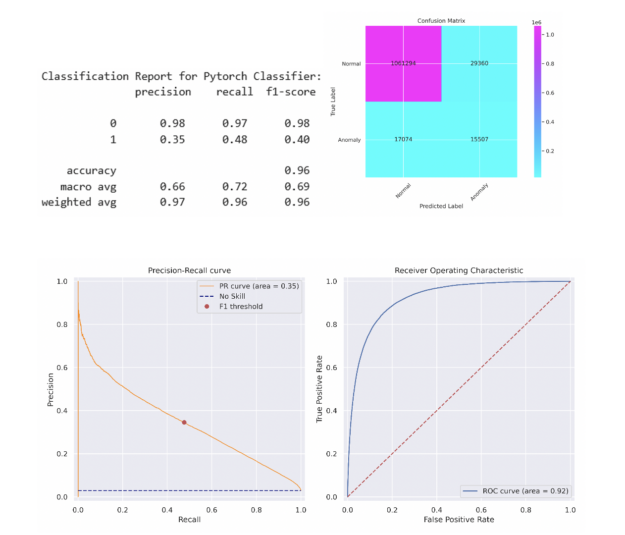
For simplicity, we opted for a 5-layer Multi-Layer Perception (MLP) neural network with 512 neurons Linear layer, PReLU, Batch Normalization, and Dropout. The simple MLP is able to match the XGBoost model’s performance on the test set. A more sophisticated model may exceed this performance. The same method was applied to find the threshold yielding the maximum F1 score on the train set before applying this threshold to the test set. The classification report and confusion matrix are described below and a similar PR curve and ROC curves are presented in Figure 5.
Explainability for Machine Learning and Deep Learning
Now that we are confident of our model for predictions, it is important to understand more about how and why it works. Shapley values can be computed with SHAP and Captum for both ML and DL models. For the SHAP package, it is easy to retrieve Shapley values for explaining our XGBoost ML model per the code snippet below:
 expl = shap.TreeExplainer(model)
 shap_values = expl.shap_values(X_test)
 shap.summary_plot(shap_values, X_test.to_pandas(), sort=False, show=False)
 plt.tight_layout()
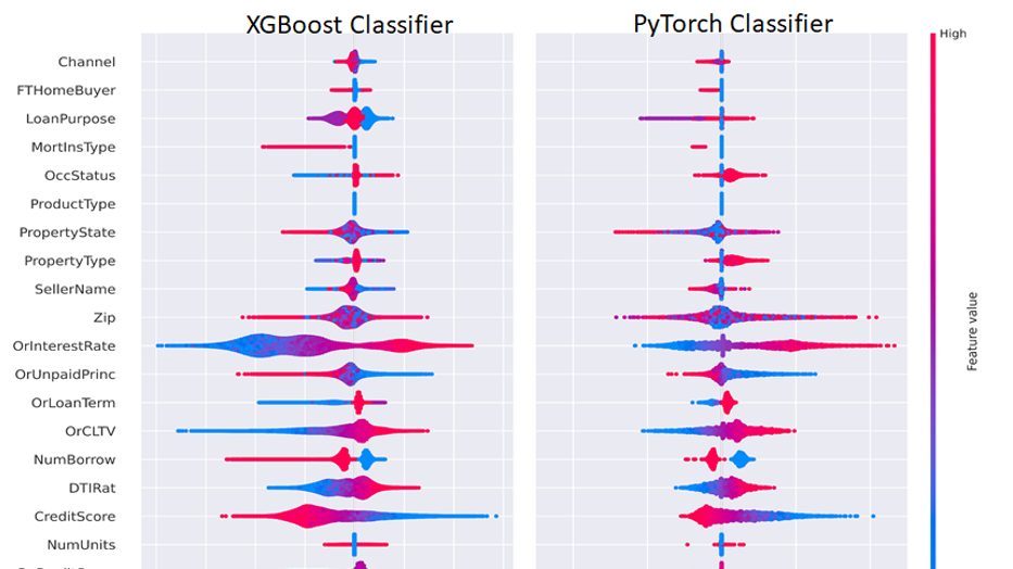
The PyTorch DL Shapley values were calculated using the Captum GradientShap method and plotted using the code below, passing the Shapley values into the SHAP summary_plot() method. We separated out positive and negative categorical and continuous variables to enable visualization of one distinct class only or for both classes, which are depicted in Figure 6.
from captum.attr import GradientShap
Gradshap = GradientShap(model)
attr_gs, delta = gradshap.attribute((torch.cat([pos_cats, neg_cats], dim=0),
                   torch.cat([pos_conts, neg_conts], dim=0)),
                   baselines=(torch.zeros_like(neg_cats, device=device),
                   torch.zeros_like(neg_conts, device=device)), n_samples=200,
                   return_convergence_delta=True)
df = DataFrame(cp.asarray(torch.cat([torch.cat([pos_cats, pos_conts], dim=1),
               torch.cat([neg_cats, neg_conts], dim=1)], dim=0)))
df.columns = CATEGORICAL_COLUMNS + CONTINUOUS_COLUMNS
svals = cp.asnumpy(torch.cat(attr_gs, dim=1))
shap.summary_plot(svals,
                  df[CATEGORICAL_COLUMNS+CONTINUOUS_COLUMNS].to_pandas(),
                  sort=False, show=False)
plt.tight_layout()
In general, we would like to explain a single prediction and interpret how the features led to that prediction. The Shapley feature explanations sum up to the prediction for a single row, and we can aggregate across rows to explain model predictions in bulk. For regulatory purposes, this means that a model can provide a human-interpretable explanation for any output, favorable, or adverse. Anyone who holds a mortgage or works in the debt instrument domain can recognize these familiar factors.
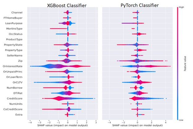
Figure 6 depicts both ML and DL Shapley values side by side. We can interpret Figure 6 in the following manner by considering the CreditScore and Interest Rate (OrInterestRate) features as an example. The red portion of the CreditScore feature indicates higher credit scores as mentioned in the legend on the right on the plot with higher feature value as red and lower feature value as blue. For CreditScore points clustered on the negative x-axis corresponding to negative SHAP values contributing to the negative or non-delinquent class suggesting that people with high credit scores are less likely to be delinquent. Symmetrically, blue (low) values for CreditScore are on the positive x-axis or positive Shapley values, indicating a contribution to the positive or delinquent class.
A similar yet opposite interpretation can be applied with the OrInterestRate feature: low (blue) interest rates yield negative Shapley values and are associated with lower delinquency rates and this makes intuitive sense as lower rates mean lower mortgage payments. Some features may be less clear and provide an opportunity for the Data Scientist or Machine Learning engineer to improve a model. For example, in our simple MLP model, we concatenated the factorized categorical features with the continuous features before passing into the MLP. An improvement to this model may be to use categorical embeddings, which could both improve model performance and enhance explainability as well. In this way, a Data Scientist or Machine Learning Engineer can try to optimize both model explainability and performance.
GPU-Acceleration results
Figures 7 and 8 focus on the test of the time required to read the input datasets, merge the two datasets, as well as the DL inference step on an NVIDIA Ampere A100 GPU when compared to an Ice Lake 24 core dual CPU. As Table 1 shows, there are solid speed ups in every step.
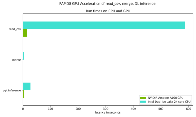
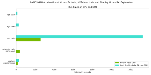
Table 1 quantifies the speedups illustrated in Figures 7 and 8, and underscores the benefit of GPU-acceleration.
| CPU only | NVIDIA Ampere A100 40GB GPU | Speed up Factor | |
| Read cvs files | 587.0 sec | 15.3 sec | 38X |
| merge | 4.6 sec | 0.04 sec | 115X |
| PyTorch inference | 27.7 sec | 4.3 sec | 6X |
| XGBoost train | 134.0 sec. | 10.7 sec | 12.5X |
| XGBoost shap | 265.0 sec | 9.2 sec | 29X |
| PyTorch train | 13314.6 sec | 2567.3 sec | 5X |
| PyTorch train with NVTabular | NA | 382.2 sec | 6X over PyTorch train w/GPU |
| Captum GradientShap | 289.1 sec | 166.8 sec | 2x |
In this post, we have expanded on a related earlier post, discussing credit default risk prediction with deep learning and discussed:
- How to use RAPIDS to GPU-accelerate the complete default analytics workflow
- How to apply the XGBoost implementation inside of RAPIDS with GPUs
- How to apply the PyTorch Deep Learning library to tabular data with GPUs
- How to use the NVIDIA NVTabular package for PyTorch DL on GPU to obtain 6x faster run-time performance simply by changing the Data Loader.
- How to access explainable predictions with the Shap and Captum packages with GPUs and using these explainable results for further model improvements.
We recommend the following steps:
- Visit the site http://ngc.nvidia.com for the NVIDIA GPU Cloud repository of containers to help build AI solutions available.
- Review or attend the most recent NVIDIA Global Technology Conference to share ideas and technology solutions.
- For more information, e-mail one of the authors listed.
