
Today’s machine learning (ML) solutions are complex and rarely use just a single model. Training models effectively requires large, diverse datasets that may require multiple models to predict effectively. Also, deploying complex multi-model ML solutions in production can be a challenging task. A common example is when compatibility issues with different frameworks can lead to delayed insights.
A solution that easily serves various combinations of deep neural nets and tree-based models and that is framework-agnostic would help simplify deployment and scale ML solutions as they take on multiple layers.
In this post, I discuss how to leverage the versatility of NVIDIA software to handle different types of models and integrate them into your application. I demonstrate how NVIDIA RAPIDS supports data preparation and ML training for large datasets and how NVIDIA Triton Inference Server seamlessly serves both deep neural nets by PyTorch and tree-based models by XGBoost when predicting credit default.
Using the American Express Default Prediction competition as an example, I explain how the multi-model solution can be deployed on either a GPU or a CPU. GPU deployment results in significantly faster inference times. This solution was one of the top 10 solutions out of 4,874 teams in the Kaggle American Express Default Prediction competition.
Future credit default predictions
Credit default prediction is central to managing risk in a consumer lending business. American Express, the largest payment card issuer in the world, provided an industrial-scale dataset that includes time-series behavioral data and anonymized customer profile information. This dataset is highly representative of real-world scenarios: it is large, contains both numerical and categorical columns, and presents a time-series problem.
The key to solving this business problem successfully is to uncover the temporal patterns within the data.
Why focus on trees and neural nets?
Tree-based models and deep neural networks are widely considered to be the most popular choices for ML practitioners.
Tree-based models, such as XGBoost, are mostly used for tabular datasets because they can handle noisy, redundant features and make it easy to interpret and understand the logic behind the predictions.
Deep neural networks, on the other hand, excel at learning long-term temporal dependencies and sequential patterns in data. They also can automatically extract features from raw data. Recently, deep neural networks have been widely used to generate high-quality new data, by exploiting their ability to learn the distribution from the existing data.
Now, I describe how my team used this technique in our American Express Default Fault Prediction solution.
Essential tools for data preparation and deployment
When you’re preparing a complex ML model, there are many steps to prepare, train, and deploy an effective model. RAPIDS and Triton Inference Server both support key phases in the ML process.
RAPIDS is a suite of open-source software libraries and APIs designed to accelerate data science workflows on GPUs. It includes a variety of tools and libraries for data preprocessing, ML, and visualization. In this case, it supports data preprocessing and exploratory data analysis at the beginning of the workflow.
To support deployment, NVIDIA Triton is a high-performance, multi-model inference server supporting both GPU and CPU that enables the easy deployment of models from a variety of frameworks, such as TensorFlow, PyTorch, and ONNX.
NVIDIA Triton supports tree-based models such as XGBoost, LightGBM, and more through its Forest Inference Library backend. This made it a great fit for the model that we were coding.
Problem overview
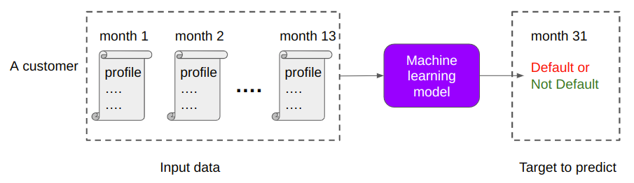
The aim is to predict if a customer will default on their credit card balance in the future, using their past monthly customer profile data. The binary target variable, default or no default, is determined by whether a customer pays back their outstanding credit card balance within 120 days of the statement date.
Figure 1 shows an overview of the problem and dataset, highlighting the key aspects of credit default prediction and the characteristics of the dataset. The test dataset is massive with 900K customers, 11M rows, and 191 columns, including both numerical and categorical features.
The goal was to create a model that can predict the categorical binary variable based on the other variables in the dataset and a mission-critical time value to manage. Before modeling, this large dataset requires significant feature engineering, making it an ideal candidate for data preparation with RAPIDS cuDF. The size of the dataset poses further challenges for real-time inferencing, which the high-performance NVIDIA Triton server addresses.
Approach
We broke the model development process into a series of steps:
- Dataset preparation
- Feature engineering
- Dataset exploration
- Autoregressive recursive neural network (RNN) model
- Dataset performance
Dataset preparation
The given American Express data is a time series consisting of multiple profiles of a customer sorted by the customer ID and timestamp:
- Each row in the dataset represents a customer’s profile for 1 month.
- Each customer has 13 consecutive rows in the data, which represent their profiles in 13 consecutive months.
- There are 214 columns in the data.
- Columns are anonymized, except for
customer_idandmonth, and fall into the following general categories: Delinquency, Spend, Payment, Balance, Risk
Table 1 summarizes the number of columns in each category. There is no information on what each column means other than its category. These anonymized columns are mostly floating-point numbers.
| customer_id | month | Delinquency | Spend | Payment | Balance | Risk | |
| # of columns | 1 | 1 | 106 | 25 | 10 | 43 | 28 |
For training data, the ground truths, default or not, are stored in another tabular data where each customer corresponds to one row. There are two columns: customer_id and default.
Feature engineering with RAPIDS cuDF
The project began with feature engineering to prepare the time-series dataset for the model. Time-series data notoriously requires massaging and becomes unwieldy for CPU-powered data science solutions. To run the data preparation efficiently for this phase, we harnessed the power of GPUs using RAPIDS cuDF.
We focused on slimming down the dataset to the most important data points by reducing the number of months for each customer profile to the last month in the set. The last month has the highest relevance in predicting future default events and reduces the number of rows to 900K. This is quickly done by drop_duplicates(keep=’last’) in cuDF.
RAPIDS cuDF can further help accelerate by creating differential and aggregate features for each customer_id value. While RAPIDS cuDF was used to engineer additional features in the preceding notebook, I disregarded those to maintain the simplicity of this single-GPU walkthrough.
Exploring the dataset
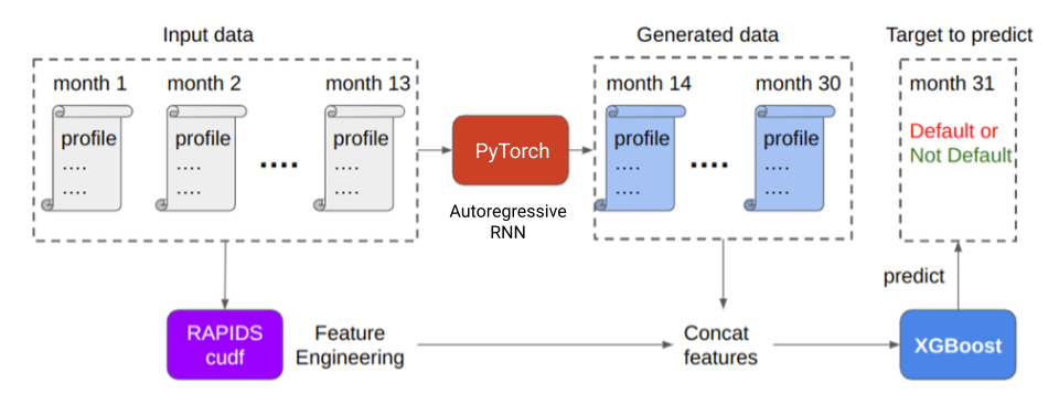
Each customer profile’s features were measured through month 13, while the date of default checking was month 31. Given the 17-month time gap in the dataset for defaulting customers, the team generated new customer profiles for the missing months (months 14 to months 30) to improve the model’s prediction rate. The team was inspired to implement the autoregressive RNN technique after exploring the data visually.
For more information about identifying the autoregressive RNN technique, see the Amex EDA Evolvement of Numeric Features Over Time notebook.
When exploring the dataset, the team visualized the data in a chart. Figure 3 plots the trends of a subset of columns over time. The x-axis is the month, and the y-axis shows the column name.
For example, the top-left subplot shows how column D_53, the 53rd column of the delinquency category, varies over months. The red dashed lines are the averaged values of column D_53 of positive samples, where Default=True and the green solid lines are averaged values of negative samples, respectively.
For most columns, there are obvious temporal patterns. A model can be trained to extrapolate and predict future values of columns. With this model, generating additional values for the dataset helps improve the model’s predictability.
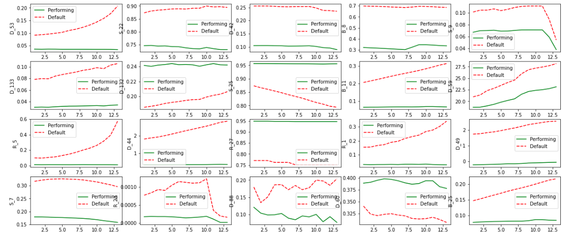
When you’re planning for enhancing the dataset, another key is that the patterns can be different for each column. Linear trends, nonlinear trends, wiggles, and more variations are all observable. The data generation model must be versatile, flexible to learn, and generalize all these different patterns.
Generating new profiles with the autoregressive RNN model
Based on these data characteristics, our team proposed an autoregressive RNN model to learn all these patterns simultaneously. Autoregressive means that the output of the current time step is the input of the next time step. Figure 4 shows how autoregressive generation works.
The input of the RNN model is the customer’s profile for the current month, including all 214 columns. The output of the RNN model is the predicted customer profile for the next month. The autoregressive RNN used in this approach is trained in a self-supervised manner, meaning it only employs customer profiles for training and does not require the “default or not” target column.
This self-supervised training to enhance datasets enables you to use a large amount of unlabeled data—a significant advantage in real-world applications as labeled data is often difficult and expensive to obtain.
Performance of the new dataset
The RNN can accurately predict future profiles. The root of the mean squared error is used between the ground truth profiles and predicted profiles. Compare the RNN against a simple baseline and assume that future profiles are the same as the last observed profile.
| Autoregressive RNN | Last observed profile baseline | |
| RMSE of all 214 columns | 0.019 | 0.03 |
In Table 2, the RNN reduced RMSE from 0.03 to 0.019 (a 33% improvement). This is a significant enhancement to the original dataset.
Figure 2 showed that the last step to producing the dataset for training is to combine the last profiles and generated profiles into one matrix. Do this using the joins function in RAPIDS cuDF and feed them to the downstream XGBoost classifier to predict defaults. The generated profiles greatly enhance the performance of the model.
Table 3 shows that, by combining the most recent profiles and generated future profiles, the XGBoost classifier can more accurately predict future default by 0.003. This is a significant improvement for default detection problems. Such improvement could move the solution rank up by hundreds of places in the American Express default prediction competition!
| xgb trained on last profiles | xgb trained on last profiles and autoregressive RNN-generated profiles | |
| American Express metric for predicting default | 0.7797 | 0.7830 |
Deploy models to Triton Inference Server
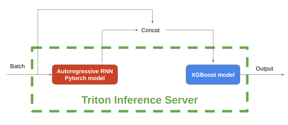
Figure 5 shows that, during inference, NVIDIA Triton Inference Server enables the hosting of both the autoregressive RNN model implemented in PyTorch and the tree-based models implemented in XGBoost, on either CPU or GPU.
First, save the pretrained PyTorch RNN models and XGBoost models in separate folders with correct folder hierarchies. Next, write configuration files for each model. The PyTorch model processes the batch of input data to generate the future profiles, after which the concatenated profiles are input into the XGBoost model for further inference.
In under 6 seconds, 115K customer profiles have been inferred with this rnn-xgb pipeline on a single GPU.
The inference time is blazing fast even with this complicated model pipeline including autoregressive RNN for 13 time-steps and XGBoost for classification. Running the NVIDIA Triton Inference Server pipeline on 11.3 million American Express customer profiles takes only 45 seconds on a single NVIDIA V100 GPU.
Summary
The proposed solution for credit default prediction shown in this post successfully leverages the power of both deep neural nets and tree models to improve the accuracy of predictions by supplementing data.
Data processing of the time-series data was easier and faster with RAPIDS cuDF. The deployment of the models was made seamless with Triton Inference Server, which can host both deep neural nets and tree models on either CPU or GPU. This makes it a powerful tool for real-time inference.
This demo also highlights the potential of applying the high-performance computing power of GPUs and Triton Inference Server in credit default prediction, opening avenues for further exploration and improvement in the financial services field.
Here are the notebooks used in this post:
