cuTENSOR 2.0: A Comprehensive Guide for Accelerating Tensor Computations

NVIDIA cuTENSOR is a CUDA math library that provides optimized implementations of tensor operations where tensors are dense, multi-dimensional arrays or array slices. The release of cuTENSOR 2.0 represents a major update—in both functionality and performance—over its predecessor. This version reimagines its APIs to be more expressive, including advanced just-in-time compilation capabilities all with the latest and greatest performance that can be achieved on the NVIDIA Ampere and NVIDIA Hopper GPU architectures.

This post introduces the cuTENSOR 2.0 library and how to use its operations. For more information, see the next post in the series, cuTENSOR 2.0: Performance and Applications.

While tensor operations might seem exotic at first glance, they describe many naturally occurring algorithms. In particular, such operations are ubiquitous in machine learning and quantum chemistry. 

If you already work with NVIDIA cuBLAS, or BLAS in general, the three routines that cuTENSOR provides may already seem familiar to you: 

• The elementwise API corresponds to level-1 BLAS (vector-vector operations)
• The reduction API corresponds to level-2 BLAS (matrix-vector operations)
• The contraction API corresponds to level-3 BLAS (matrix-matrix operations)

The key difference is that cuTENSOR extends those operations to multiple dimensions. cuTENSOR enables you to avoid worrying about performance optimization for these operations and instead rely on ready-made accelerated routines.

The cuTENSOR benefits and advances are available for your use not only from your CUDA code, but also from any of the many tools that include support for it already, today. 

• Fortran developers can benefit from the cuTENSOR Fortran API bindings available as part of the NVIDIA HPC SDK when using NVFORTRAN. 
• Python developers can access the NVIDIA GPU-accelerated tensor contractions, reductions, and elementwise computations available in cuTENSOR through CuPy.
• cuTENSOR is also available to Julia developers using Julia Lang as well. 

The selection of programs that are accelerated with cuTENSOR is constantly expanding. We also provide example code that gets you started in C++ and Python with TensorFlow and PyTorch.

In this post, we discuss the various operations that cuTENSOR supports and how to take advantage of them as a CUDA programmer. We share performance considerations and other useful tips and tricks. Finally, the sample code that we use is also available as part of the /NVIDIA/CUDALibrarySamples GitHub repository.

cuTENSOR 2.0

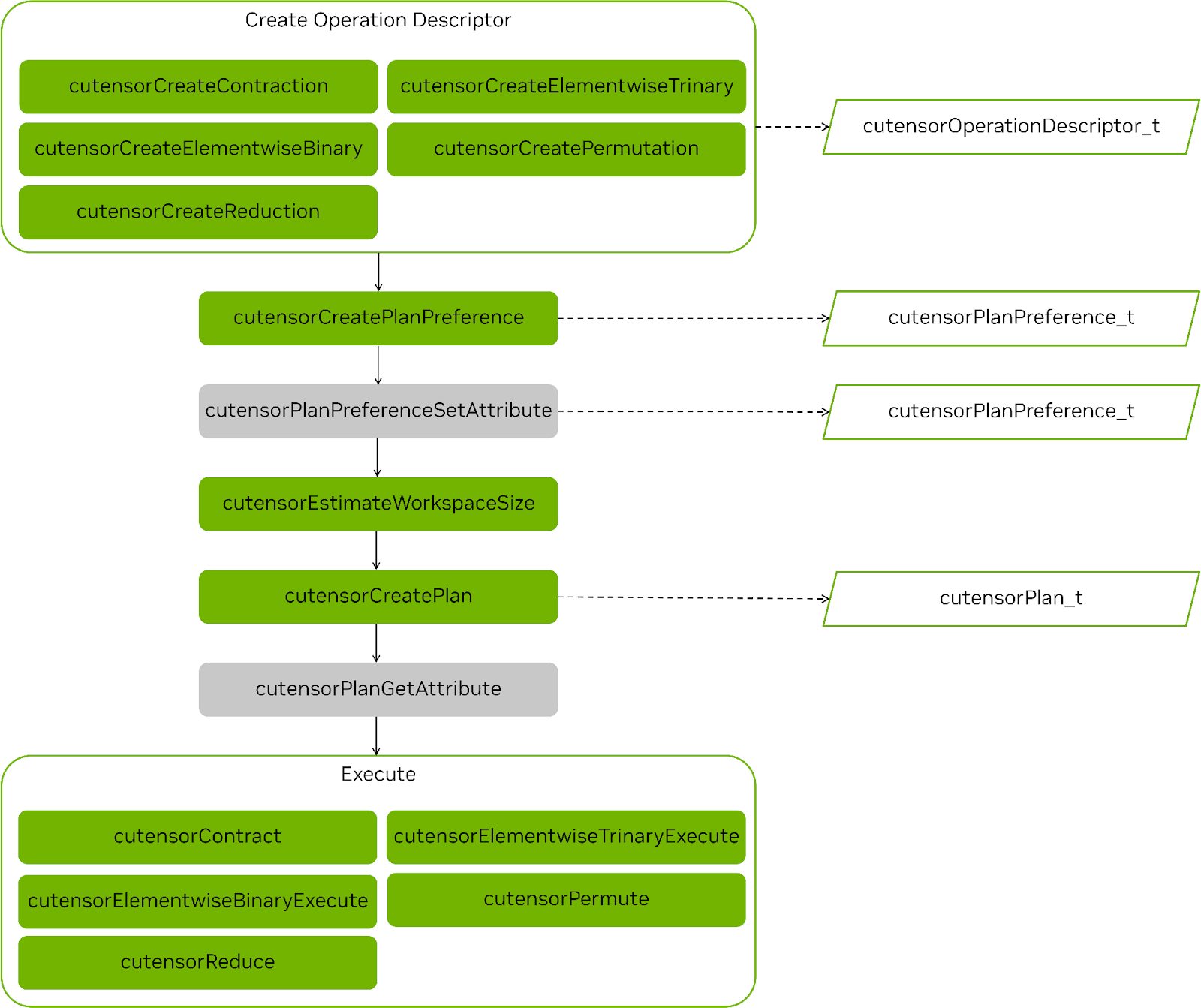
cuTENSOR 2.0 represents a major advancement over its 1.x predecessor in performance, feature support, and ease of use. We overhauled the API of elementwise operations, reductions and tensor contractions to make them coherent such that all operations follow the same multi-stage API design (Figure 1).

For the first time, cuTENSOR introduces just-in-time compilation support for tensor contractions that enable you to compile a dedicated kernel tailored to a specific tensor contraction. This feature is especially valuable for high-dimensional tensor contractions, as they are frequently encountered in quantum circuit simulations.

Tensor permutations also support padding now, enabling the output tensor to be padded along any dimension to meet any alignment requirements or to avoid predication of a subsequent kernel.

Starting with cuTENSOR 2.0, the plan cache is enabled by default. That is, instead of opt-in, its default was changed to opt-out. This helps to reduce the planning overhead in a user-friendly manner.

Finally, we made the API design between elementwise operations, reductions and tensor contractions coherent in the sense that all operations follow the same multi-stage API design as contractions, which, among other things, enables you to reuse the plan for elementwise and reduction operations.

This post solely focuses on the latest 2.0 API. For more information about how to transition from 1.x to 2.0, see Transition to cuTENSOR 2.x.

API introduction

This section introduces the key concepts behind cuTENSOR APIs and how to invoke them in your code. For more information and comprehensive examples, see the /NVIDIA/CUDALibrarySamples GitHub repo and Getting Started in the cuTENSOR documentation.

The first step is always to initialize the cuTENSOR library handle (one per thread). This enables the library to prepare for execution and do expensive setup work only one time.

cutensorStatus_t status;
cutensorHandle_t handle;

status = cutensorCreate(handle);
// [...] check status

After the handle is created, it can be reused for any of the subsequent API calls. Starting with cuTENSOR 2.0, all operations follow the same workflow:

1. Create the operation descriptors:
   1. cutensorTensorDescriptor_t to capture the physical layout of the tensor.
   2. cutensorOperationDescriptor_t to encode the operation itself.
   3. cutensorPlanPreference_t to limit the space of applicable kernels.
2. (Optional) Set the attributes of the plan preference.
3. Estimate the workspace requirement.
4. Create cutensorPlan_t to select the kernel that is used to perform the operation.
   1. Invoke the cuTENSOR performance model.
   2. Might result in a compilation step if JIT was enabled.
5. (Optional) Query the workspace that is actually used by the plan.
6. Execute the actual operation.

Figure 1 shows the steps involved in any operation and highlights the common steps.

Tensor descriptors are integral to the cuTENSOR API. They encode the following:

• Physical layout of a dense tensor:
  • Data type of the tensor elements
  • Number of dimensions (rank)
• Extent of each dimension
• Stride (linear memory) between two adjacent elements of the same dimension 
• Alignment requirement (bytes) of the corresponding data pointer (this is typically 256 bytes, matching the CUDA default alignment of cudaMalloc). 

In this post, we use the terms dimension and mode interchangeably.

This might sound abstract, so consider Figure 2. It is a three-dimensional tensor with elements numbered based on how they are arranged in memory. This tensor has an extent of three elements in each dimension. Its strides are one in the first dimension, three in the second dimension, and nine in the last dimension. This corresponds to the difference in position between two elements in that dimension.

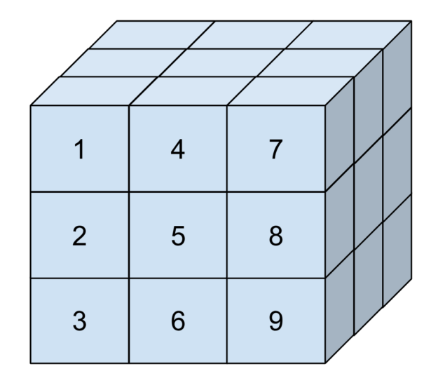
Strides enable you to represent sub-tensors (tensors that are slices of a larger tensor) by setting strides that are larger than the extents. In cuTENSOR, strides are always given in units of elements, just like extents.

For example, to express the tensor from the figure, you would invoke the following code:

int64_t extents[] = {3, 3, 3};
int64_t strides[] = {1, 3, 9};
uint32_t alignment = 256; // bytes (default of cudaMalloc)
cutensorTensorDescriptor_t tensor_desc;
status = cutensorCreateTensorDescriptor(handle, tensor_desc,
                                        3 /*num_modes*/, 
                                        extents, strides, 
                                        CUTENSOR_R_32F, alignment);

You could also pass a NULL pointer instead of strides. In that case, cuTENSOR would automatically deduce the strides from the extents for a dense tensor, assuming a generalized column-major memory layout. That is, strides increase from left to right, with the left-most mode having a stride of one. Any other layout, including generalized row-major, can be achieved by providing the appropriate strides.

Strides can also be used to access sub-tensors. For instance, the following code example encodes a two-dimensional, non-contiguous horizontal plane of the previous tensor:

int64_t extents_slice[] = {3, 3};
int64_t strides_slice[] = {3, 9};
status = cutensorCreateTensorDescriptor(handle, tensor_desc,
                                      2 /*num_modes*/,
                                      extents_slice, strides,
                                      CUTENSOR_R_32F, alignment);

Einsum notation

A common design decision between the cuTENSOR elementwise, reduction and contraction APIs is that they all adhere to the einsum notation. Each dimension, also referred to as a mode, is given a unique label. Tensor operations, such as permutations and contractions, can be expressed in an user-friendly manner by simply permuting or omitting modes. Modes that don’t appear in the output are contracted. For more information, see torch.einsum in the PyTorch documentation.

For example, permuting a four dimensional tensor that is stored in the layout to the format can be expressed as follows:

The letters before the denote the modes of the input tensor and the letters behind it denote modes of the output tensor. 

Similarly, a matrix-matrix multiplication can be expressed as , where the dimension is contracted. We use this notation throughout the upcoming sections.

Contraction

Tensor contractions can be thought of as the higher-dimensional equivalent of matrix-matrix multiplications. The only difference is that the operands are multi-dimensional instead of just two-dimensional matrices. For more information about the exact equation, see cuTENSOR Functions.

In this post, we show the usage of the cuTENSOR API using the example of a tensor contraction operation. However, the other APIs behave similarly. From start to finish, the following steps are required to implement this:

1. Create an operation descriptor.
2. Create a plan preference.
3. Query the workspace size.
4. Create a plan.
5. (Optional) Query the exact workspace size usage.
6. Execute the contraction.

Create an operation descriptor

As outlined earlier, you start by creating tensor descriptors. When that is done, proceed to encoding the actual contraction:

cutensorComputeDescriptor_t descCompute = CUTENSOR_COMPUTE_DESC_32F;
cutensorOperationDescriptor_t desc;
cutensorCreateContraction(handle, &desc,
        descA, {‘a’,’b’,’k’},  /* unary op A*/ CUTENSOR_OP_IDENTITY,
        descB, {‘m’,’k’,’n’},  /* unary op B*/ CUTENSOR_OP_IDENTITY,
        descC, {‘m’,’a’,’n’,’b’},  /* unary op C*/ CUTENSOR_OP_IDENTITY,
        descC, {‘m’,’a’,’n’,’b’},
        descCompute)

The code example encodes a tensor contraction of two three-dimensional inputs to create a four-dimensional output;. The API resembles the corresponding einsum notation:

Performance guidelines

This section assumes a generalized column-major data layout where the left-most mode has the smallest stride. 

While cuTENSOR can work with modes that are provided in any order, the order can have an impact on performance. We generally recommend the following performance guidelines:

• Try to arrange the modes (with regard to increasing strides) similarly in all tensors. For instance, instead of .
• Try to keep batched modes as the slowest-varying modes (that is, with the largest strides). For instance, instead of .
• Try to keep the extent of the fastest-varying mode (stride-one mode) as large as possible.

Create a plan preference

The next step is to specify the space of applicable kernels to the problem by creating a cutensorPlanPreferrence_t object. For instance, you can use the plan preference to fix the cutensorAlgo_t object that should be used, specify the concrete kernel if you want to implement autotuning or enable just-in-time compilation.

cutensorAlgo_t algo = CUTENSOR_ALGO_DEFAULT;
cutensorJitMode_t jitMode = CUTENSOR_JIT_MODE_NONE;
cutensorPlanPreference_t planPref;
cutensorCreatePlanPreference(handle,
                             &planPref,
                             algo, jitMode);

Any plan created with this plan preference relies on the cuTENSOR performance model to pick the most suitable pre-compiled kernel: CUTENSOR_ALGO_DEFAULT. In this case, you’ve disabled JIT compilation. 

As we briefly mentioned earlier, JIT compilation enables generating a dedicated kernel for the specific operation at runtime leading to significant performance improvement. To take advantage of the cuTENSOR JIT capabilities, set jitMode = CUTENSOR_JIT_MODE_DEFAULT. For more information, see the JIT compilation and performance section later in this post.

Query the workspace size

Now that you’ve initialized the contraction descriptor and created a plan preference, you can proceed to estimate the workspace size requirement using cutensorEstimateWorkspaceSize. 

The API gives you a choice over the desired workspace estimate through cutensorWorksizePreference_t. CUTENSOR_WORKSPACE_DEFAULT is a good default value as it aims to attain high performance while also reducing the workspace requirement. If memory footprint is not a concern, then CUTENSOR_WORKSPACE_MAX might be a better choice.

uint64_t workspaceSizeEstimate = 0;
cutensorWorksizePreference_t workspacePref = CUTENSOR_WORKSPACE_DEFAULT;
cutensorEstimateWorkspaceSize(handle,
                                      	desc,
                                      	planPref,
                                      	workspacePref,
                                      	&workspaceSizeEstimate);

Create a plan

The next step is to create the actual plan, which encodes the execution of the operation and selects the kernel. This step involves querying the cuTENSOR performance model and is typically the most time-consuming step of the setup phase. This is why, starting with cuTENSOR 2.0.0, it is automatically cached in a user-controlled cache. For more information, see the Plan cache and incremental autotuning section later in this post. 

Creating the plan is also the step that, if enabled, causes a kernel to be just-in-time compiled.

cutensorPlan_t plan;
cutensorCreatePlan(handle,	&plan, desc, planPref, workspaceSizeEstimate);

cutensorCreatePlan accepts a workspace size limit as input (in this case, it is workspaceSizeEstimate) and guarantees that the created plan does not exceed this limit.

(Optional) Query the exact workspace size usage

Starting with cuTENSOR 2.0.0, it is possible to query the created plan for the exact amount of workspace that it actually uses. While this step is optional, we recommend it to reduce the required workspace size.

uint64_t actualWorkspaceSize = 0;
cutensorPlanGetAttribute(handle,
    	plan,
    	CUTENSOR_PLAN_REQUIRED_WORKSPACE,
    	&actualWorkspaceSize,
    	sizeof(actualWorkspaceSize));

Execute the contraction

All that remains is to execute the contraction and provide the appropriate data pointers that must be accessible by the GPU. For more information about when data remains on the host, see Extending Block-Cyclic Tensors for Multi-GPU with NVIDIA cuTENSORMg.

cutensorContract(handle,
                    plan,
                    (void*) &alpha, A_d, B_d,
                    (void*) &beta, C_d, C_d,
                    work, actualWorkspaceSize, stream);

Elementwise operations

Elementwise operations are structurally the simplest operations in cuTENSOR. Elementwise mean operations where the size of the participating tensors is not reduced in any way. That is, you perform an operation in an element-by-element manner. Common elementwise operations include copying a tensor, permuting a tensor, adding tensors or elementwise multiplying them (also known as the Hadamard product). 

Depending on the number of input tensors, cuTENSOR offers three elementwise APIs:

• cutensorCreatePermute for one input tensor
• cutensorCreateElementwiseBinary for two input tensors
• cutensorCreateElementwiseTrinary for three input tensors

As an example, consider a permutation. Here, tensors A (source) and B (destination) are rank-4 tensors and you permute their modes from NHWC to NCHW. The creation of the operation descriptor can be implemented as follows. Compare with steps 1 and 6 from the previous section.

float alpha = 1.0f;
cutensorOperator_t op = CUTENSOR_OP_IDENTITY;
cutensorComputeDescriptor_t descCompute = CUTENSOR_COMPUTE_DESC_32F;
cutensorOperationDescriptor_t permuteDesc;
status = cutensorCreatePermutation(handle, &permuteDesc,
                                &alpha, descA, {‘N’, ‘H’, ‘W’, ‘C’}, op,
                                        descB, {‘N’, ‘C’, ‘H’, ‘W’},
                                descCompute, stream);
// next stages (such as plan creation) omitted …
cutensorPermute(handle, plan, &alpha, A_d, C_d, nullptr /* stream */));

This code example only highlights the differences with regard to the previous contraction example. All stages but the creation of the operation descriptor and the actual execution are identical to that of a contraction. The only exception is that elementwise operations do not require any workspace.

cuTENSOR 2.0 also offers support for padding the output tensor of a tensor permutation. This can be especially useful if alignment requirements must be met, such as enabling vectorized loads. 

The following code example outlines how an output tensor can be padded with zeros. To be precise, one element of padding is added each to the left and to the right of the fourth mode and all other modes remain non-padded.

cutensorOperationDescriptorSetAttribute(handle, permuteDesc,
                               CUTENSOR_OPERATION_DESCRIPTOR_PADDING_RIGHT,
                               {0,0,0,1},
                               sizeof(int) * 4));
cutensorOperationDescriptorSetAttribute(handle, permuteDesc,
                               CUTENSOR_OPERATION_DESCRIPTOR_PADDING_LEFT,
                               {0,0,0,1},
                               sizeof(int) * 4));
float paddingValue = 0.f;
cutensorOperationDescriptorSetAttribute(handle, permuteDesc,
                               CUTENSOR_OPERATION_DESCRIPTOR_PADDING_VALUE,
                               &paddingValue, sizeof(paddingValue));

For more information and a fully functional padding example, see the /NVIDIA/CUDALibrarySamples GitHub repo.

Reduction

The cuTENSOR tensor reduction operation takes a single tensor as input and reduces the number of dimensions in that tensor using a reduction operation: summation, multiplication, maximum, or minimum. For more information, see cutensorOperator-t. 

Similar to contractions and elementwise operations, tensor reductions also use the same multi-stage API. This API example is limited to the parts that differ.

cutensorOperationDescriptor_t desc;
cutensorOperator_t opReduce = CUTENSOR_OP_ADD;
cutensorCreateReduction(handle, &desc,
             	descA, {‘a’, ‘b’, ‘c’}, CUTENSOR_OP_IDENTITY,
             	descC, {‘b’, ‘a’,},  CUTENSOR_OP_IDENTITY,
             	descC, {‘b’, ‘a’,},
             	opReduce, descCompute);
// next stages (such as plan creation) omitted …
cutensorReduce(handle, plan,
               (const void*)&alpha, A_d,
               (const void*)&beta, C_d,
                                   	C_d,
                work, actualWorkspaceSize, stream);

The input tensor doesn’t have to be fully reduced to a scalar but some modes can still remain. Also, there’s no constraint on the exact order of modes either, which effectively fuses permutations and reductions into a single kernel. For instance, the tensor reduction not only contracts the mode but also changes the order of the remaining modes.

Just-in-time compilation

As we mentioned in the Contraction section earlier in this post, cuTENSOR 2.0 introduced just-in-time compilation support for tensor contractions to produce dedicated kernels tailored to a given tensor contraction at runtime. This is especially valuable to provide the best possible performance for challenging tensor contractions, such as high-dimensional tensor contractions, where pre-built kernels may not be as performant. 

Just-in-time compilation can be enabled by passing CUTENSOR_JIT_MODE_DEFAULT to cutensorCreatePlanPreference for the relevant tensor contraction operation.

cutensorAlgo_t algo = CUTENSOR_ALGO_DEFAULT;
cutensorJitMode_t jitMode = CUTENSOR_JIT_MODE_DEFAULT;
cutensorPlanPreference_t planPref;
cutensorCreatePlanPreference(handle,
                             &planPref,
                             algo, jitMode);

The actual compilation of the kernel is then performed using NVIDIA nvrtc and occurs upon the first call to cutensorCreatePlan at runtime. The successfully compiled kernel is then automatically added to an internal kernel cache such that any subsequent calls for the same operation descriptor and plan preference would just result in cache look-up rather than a recompilation.

To further amortize the overhead of JIT compilation, cuTENSOR provides the cutensorReadKernelCacheFromFile and cutensorWriteKernelCacheToFile APIs that enable you to read and write the internal kernel cache to a file such that it can be reused across multiple program executions.

cutensorReadKernelCacheFromFile(handle, "kernelCache.bin");
// execution (possibly with JIT-compilation enabled) omitted…
cutensorWriteKernelCacheToFile(handle, "kernelCache.bin");

For more information, see Just-In-Time Compilation.

Plan cache and incremental autotuning

Planning is the most time-consuming setup stage as it invokes the cuTENSOR performance model. It is a good practice to store a plan and reuse it multiple times with potentially different data pointers. 

However, given that such reuse may not always be possible or may be time consuming to implement on the user side, cuTENSOR 2.0 employs a software-managed plan cache per library handle that is activated by default. You can still opt-out by using CUTENSOR_CACHE_MODE_NONE on an operation-by-operation basis.

The plan cache reduces the time that cutensorCreatePlan takes by ~10x.

The plan cache employs a least recently used (LRU) eviction policy and has a default capacity of 64 entries. Ideally, you’d want the cache to have the same or higher capacity as the number of unique tensor contractions. cuTENSOR provides the option to change the cache capacity as follows:

int32_t numEntries = 128;
cutensorHandleResizePlanCachelines(&handle, numEntries);

Similar to the kernel cache, the plan cache can also be serialized from and to disc so it can be reused across program executions:

uint32_t numCachelines = 0;
cutensorHandleReadPlanCacheFromFile(handle, "./planCache.bin", &numCachelines);
// execution (possibly with JIT-compilation enabled) omitted…
cutensorHandleWritePlanCacheToFile(handle, "./planCache.bin");

Incremental autotuning is an opt-in feature of the plan cache. It enables successive invocations of the same operation, with potentially different data pointers, to be performed by different candidates or kernels. After a user-defined number of candidates has been explored, the fastest one is stored in the plan cache and used thereafter for the specific operation. 

Compared to other methods of autotuning, incremental autotuning using the plan cache has the following advantages:

• It does not require other modifications to the existing code from the user’s perspective, other than enabling the feature. The measurement overhead is also minimized in that it does not use a timing loop or synchronization.
• Candidates are evaluated at a point in time where hardware caches are in a state that matches the production environment. That is, the hardware cache state reflects the real-world situation.

Incremental autotuning can be enabled during plan preference creation, as follows:

const cutensorAutotuneMode_t autotuneMode = CUTENSOR_AUTOTUNE_MODE_INCREMENTAL;
cutensorPlanPreferenceSetAttribute(
	&handle,
	&find,
	CUTENSOR_PLAN_PREFERENCE_AUTOTUNE_MODE_MODE,
	&autotuneMode ,
	sizeof(cutensorAutotuneMode_t));

// Optionally, also set the maximum number of candidates to explore
const uint32_t incCount = 4;
cutensorPlanPreferenceSetAttribute(
	&handle,
	&find,
	CUTENSOR_PLAN_PREFERENCE_INCREMENTAL_COUNT,
	&incCount,
	sizeof(uint32_t));

For more information about the cuTENSOR plan cache and incremental autotuning features, see Plan Cache.

Multi-GPU support

For more information, see Extending Block-Cyclic Tensors for Multi-GPU with NVIDIA cuTENSORMg.

Summary

When working with dense tensors, cuTENSOR provides a comprehensive collection of routines that make your life as a CUDA developer easier and enable you to achieve high performance without having to worry about low-level performance optimizations. Many of the algorithms that you would want to apply to tensors can be expressed using the existing cuTENSOR routines.

As a CUDA library user, you can also benefit from automatic performance-portable code for any future NVIDIA architecture and other performance improvements, as we continuously optimize the cuTENSOR library.

For more information, see cuTENSOR 2.0: Applications and Performance.

Get Started with cuTENSOR 2.0

Get started with cuTENSOR 2.0.

Dive deeper and ask questions about cuTENSOR 2.0 in the Developer Forums.