
While part 1 focused on the usage of the new NVIDIA cuTENSOR 2.0 CUDA math library, this post introduces a variety of usage modes beyond that, specifically usage from Python and Julia. We also demonstrate the performance of cuTENSOR based on benchmarks in a number of application domains.

PyTorch and TensorFlow
We provide the cutensor Python package, which contains PyTorch and TensorFlow bindings for an einsum style interface. The package leverages cuTENSOR and can be used similar to the PyTorch and TensorFlow native einsum implementations. For more information, see Installation.
For instance, cuTENSOR can be used as a alternative to torch.einsum as the following code example shows:
from cutensor.torch import EinsumGeneral
output =  EinsumGeneral('kc,nchw->nkhw', input_a, input_b) // similar to torch.einsum(...)
CuPy
CuPy recently added support for cuTENSOR 2.0, which makes it simple for Python developers to exploit cuTENSOR improved performance. To enable cuTENSOR as a backend for CuPy, export the CUPY_ACCELERATORS=cub,cutensor environment variable and install the correct CuPy version.
Using pip:
pip install cupy-cuda12x cutensor-cu12
Using conda:
conda install -c conda-forge cupy "cutensor>=2" cuda-version=X.Y
After cuTENSOR is enabled, it automatically accelerates the CuPy einsum function:
import cupy as cp

# tensor contraction can be accelerated by cuTENSOR
a = cp.random.random((3, 4, 5))
b = cp.random.random((4, 5, 6))
c = cp.random.random((6, 7))
out = cp.einsum(“abc,bcd,de->ae”, a, b, c)
In addition, CuPy also provides direct access to cuTENSOR lower-level APIs so that the previous einsum function can be also be expressed as follows:
import cupy as cp
import cupyx.cutensor as cutensor

alpha = 1.0
beta = 0.0
mode_a = ('a', 'b', 'c')
mode_b = ('b', 'c', 'd')
mode_c = ('d', 'e')
mode_ab = ('a', 'd')
mode_abc = ('a', 'e')
a = cp.random.random((3, 4, 5))
b = cp.random.random((4, 5, 6))
c = cp.random.random((6, 7))
ab = cp.empty((3, 6))
abc = cp.empty((3, 7))
cutensor.contraction(alpha, a, mode_a, b, mode_b, beta, ab, mode_ab)
cutensor.contraction(alpha, ab, mode_ab, c, mode_c, beta, abc, mode_abc)
Julia Lang
CUDA.jl (v.5.2.0) added support for cuTENSOR 2.0, which makes it simple for Julia developers to benefit from cuTENSOR improved performance. To use cuTENSOR in Julia, install the CUDA.jl package.
After CUDA.jl is installed, it automatically uses cuTENSOR to accelerate contractions using CuTensor objects.
using CUDA
using cuTENSOR

dimsA = (3, 4, 5)
dimsB = (4, 5, 6)
indsA = ['a', 'b', 'c']
indsB = ['b', 'c', 'd']
A = rand(Float32, (dimsA...,))
B = rand(Float32, (dimsB...,))
dA = CuArray(A)
dB = CuArray(B)
ctA = CuTensor(dA, indsA)
ctB = CuTensor(dB, indsB)

ctC = ctA * ctB      # cuTENSOR is used to perform the contraction

C, indsC = collect(ctC)
CUDA.jl also provides direct access to cuTENSOR lower-level APIs so that the previous contraction can also be expressed as follows:
using CUDA
using cuTENSOR

dimsA = (3, 4, 5)
dimsB = (4, 5, 6)
dimsC = (3, 6)
indsA = ['a', 'b', 'c']
indsB = ['b', 'c', 'd']
indsC = ['a', 'd']
A = rand(Float32, (dimsA...,))
B = rand(Float32, (dimsB...,))
C = zeros(Float32, (dimsC...,))
dA = CuArray(A)
dB = CuArray(B)
dC = CuArray(C)

alpha = rand(Float32)
beta = rand(Float32)
opA = cuTENSOR.OP_IDENTITY
opB = cuTENSOR.OP_IDENTITY
opC = cuTENSOR.OP_IDENTITY
opOut = cuTENSOR.OP_IDENTITY
comp_type = cuTENSOR.COMPUTE_DESC_TF32
plan  = cuTENSOR.plan_contraction(dA, indsA, opA,
                                                                 dB, indsB, opB,
                                                                 dC, indsC, opC, opOut;
                                                                 compute_type=comp_type)
dC = cuTENSOR.contract!(plan, alpha, dA, dB, beta, dC)
C = collect(dC)
Performance
This section takes a closer look at the performance of cuTENSOR 2.0 and compares it to other tools.
cuTENSOR 2.0.0 vs. 1.7.0
cuTENSOR 2.0.0 exhibits a noticeable speedup over its 1.x predecessor. Among the key changes responsible for this performance boost are the following:
- Improvements to the kernels
- Improvements to the performance model to select the best kernel
- Introduction of just-in-time compilation support
Figure 1 outlines the speedup of cuTENSOR 2.0.0 over cuTENSOR 1.7.0 across a wide range of tensor contractions for NVIDIA GA100 and GH100 GPUs grouped by different data types. This speedup does not include JIT.
The speedups denoted in this plot rely on CUTENSOR_ALGO_DEFAULT which invokes the cuTENSOR performance model. It is worth noting that the performance improvement is especially large for the NVIDIA Hopper architecture (GH100).
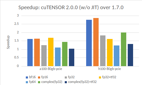
Left: NVIDIA A100 80GB PCIe; right: NVIDIA H100 80 GB PCIe. Different data types are color coded.
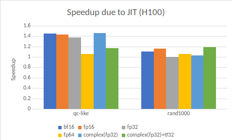
Figure 2 focuses on the performance gain solely due to just-in-time compilation. That is, it compares cuTENSOR 2.0 without JIT to cuTENSOR 2.0 with JIT on the NVIDIA GH100 GPU.
Figure 2 groups the contractions into two distinct benchmarks:
- QC-like is a benchmark that captures the structure of tensor contractions typically encountered in quantum circuit simulations with an average tensor dimensionality of 19.4.
- rand1000 is a public contraction benchmark with random contractions with an average tensor dimensionality of 4.3.
The speedup due to JIT is much larger for the QC-like benchmark. This is unsurprising as those contractions are more complicated. They often result in skewed contractions that warrant a dedicated kernel that cannot be meaningfully addressed with a fixed set of prebuilt kernels.
Quantum circuit simulation
This subsection outlines the performance improvements that cuTENSOR delivers for a tensor-network-based quantum circuit simulation of the 53-qubit Sycamore quantum circuit with a circuit depth of m=20.
We demonstrate the performance of the tensor network contraction based on two different slicing choices to restrict the size of the largest intermediate tensor to 16 GB or 32 GB. This yields vastly different contraction paths (the order in which the tensors are contracted). For more information, see Classical Simulation of Quantum Supremacy Circuits.
Ideally, you’d want to slice as few modes as possible to reduce the number of floating-point operations (FLOPs). However, this also increases the required memory, rendering some slicing options infeasible.
To be precise, PyTorch was not applicable to the better slicing option that resulted in a 32 GB intermediate tensor, due to its increased memory requirement. cuTENSOR, on the other hand, does not exhibit the same limitation, thanks to its direct contraction kernel that does not require any auxiliary memory.
We order the tensor modes identically for all frameworks to ensure an apples-to-apples comparison. For more information, see The Importance of Mode Ordering of Intermediate Tensors and Efficient Quantum Circuit Simulation by Tensor Network Methods on Modern GPUs.
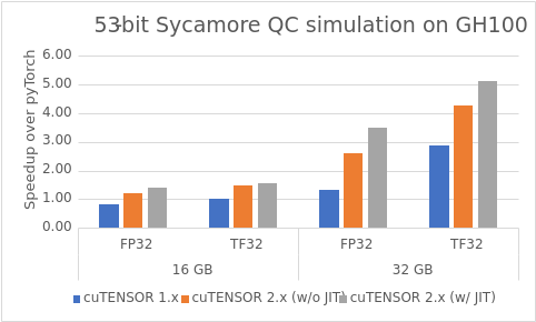
Figure 3 highlights the speedup of cuTENSOR 2.0 over PyTorch 2.1.0 for the sycamore QC simulation. It can be summarized as follows:
- cuTENSOR 2.0 consistently outperforms PyTorch.
- cuTENSOR 2.0 improves over its predecessor (similar to Figure 3)
- Just-in-time compilation improves performance even further (similar to Figure 4)
- TF32 noticeably improves performance over FP32.
- The speedups over PyTorch are especially high for the contraction path that results in a larger, 32-GB intermediate tensor. This is due to the fact that PyTorch consumes too much memory so that it is not applicable to the more computational-efficient contraction path. We compared against the best path that PyTorch is still able to compute: the path corresponding to the 16 GB intermediate.
Quantum chemistry many-body theory
Coupled cluster with single, double, and perturbative triple excitations (CCSD(T)) is a quantum chemical method renowned for its precision in calculating the electronic structures of molecules. It is often referred to as the gold standard within the realm of quantum chemistry computations, particularly for systems where the correlation of electrons is crucial.
The CCSD(T) method enhances the Hartree-Fock approach by incorporating the correlated electron movements through a series of excitation levels. In this method, the single and double electron excitations are computed in an iterative manner, while triple excitations are included through a perturbative correction that is applied non-iteratively.
This method is particularly effective for accurately predicting ground-state energies, reaction energies, and barrier heights, especially in systems with weak electron correlation. Despite its demanding computational requirements, CCSD(T) strikes a favorable balance between accuracy and computational expense, making it a popular choice in the field of computational chemistry.
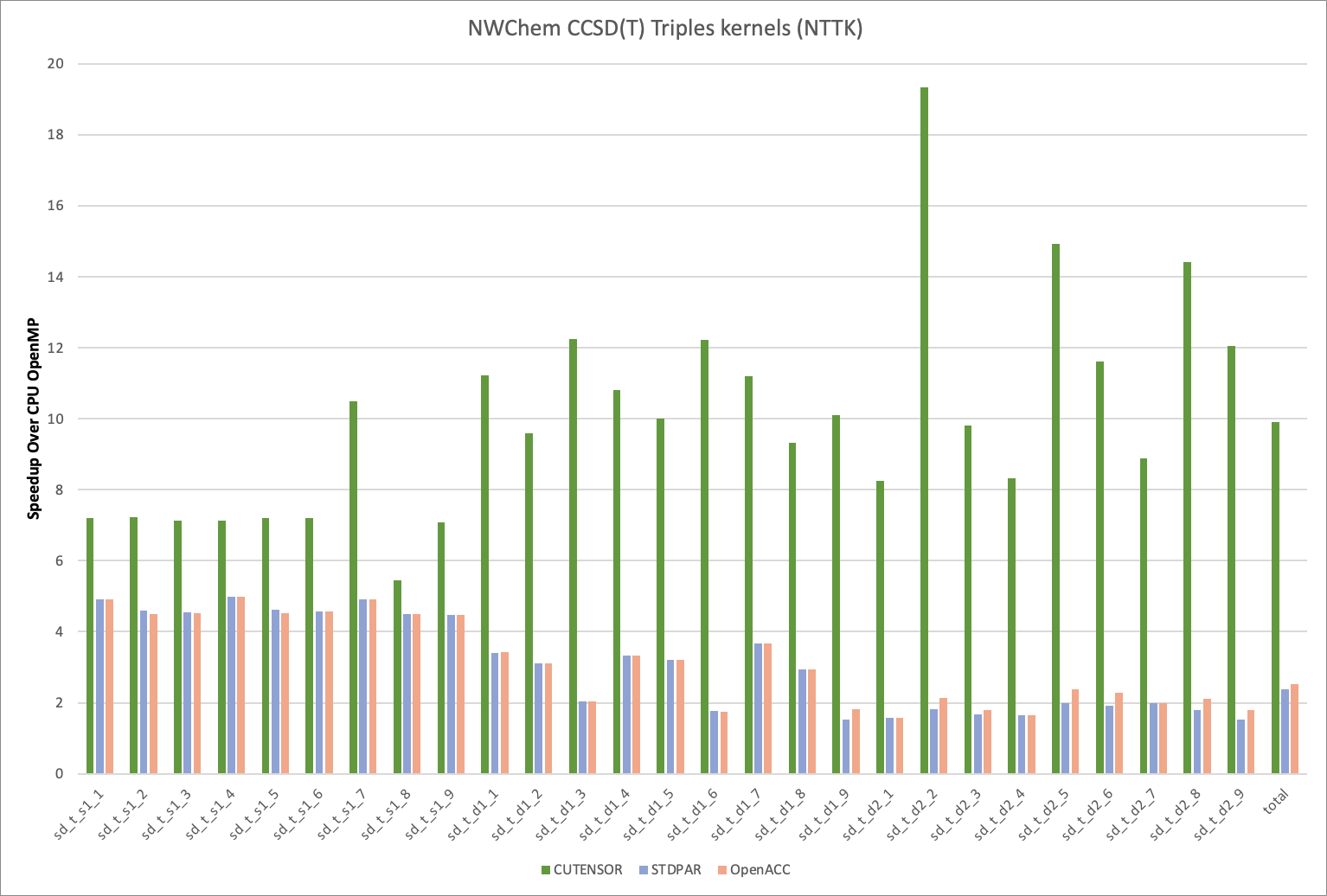
Figure 4 highlights the speedup of cuTENSOR running on an NVIDIA H100 GPU over an OpenMP-based implementation running on a 72-core NVIDIA Grace CPU. The benchmark uses NWChem TCE CCSD(T) loop-driven kernels, which are a standalone driver for the CCSD(T) triples kernels found in the NWChem Tensor Contraction Engine (TCE) module.
Get Started with cuTENSOR 2.0
If you have feature requests, such as computation routines or different compute or data types, that you would like cuTENSOR to support, please reach out to us Math-Libs-Feedback@nvidia.com.
Get started with cuTENSOR 2.0 today. Dive deeper and ask questions about cuTENSOR 2.0 in the Developer Forums.
[1] Huang, Cupjin, et al. “Classical simulation of quantum supremacy circuits.” arXiv preprint arXiv:2005.06787 (2020).
[2] Springer, Charara, Hoehnerbach. SIAM CSE’23 “The Importance of Mode Ordering of Intermediate Tensors”
[3] Pan, Feng, et al. “Efficient Quantum Circuit Simulation by Tensor Network Methods on Modern GPUs.” arXiv preprint arXiv:2310.03978 (2023).
