
After exploring the fundamentals of diffusion model sampling, parameterization, and training as explained in Generative AI Research Spotlight: Demystifying Diffusion-Based Models, our team began investigating the internals of these network architectures.
This turned out to be a frustrating exercise. Any direct attempt to improve these models tended to worsen the results. They seemed to be in a delicate, finely tuned, high-performance condition, and any change would disturb the balance. While benefits might be realized by thoroughly re-tuning the hyperparameters, the next set of improvements would require going through the whole process again.
If this tedious development loop sounds familiar to you but you don’t work directly with diffusion, read on. Our findings target universal issues and components underlying most neural networks and their training.
Rather than gritting our teeth and iterating, we decided to break the cycle and take a step back to examine the fundamentals. Why is the architecture so brittle? Are there unidentified phenomena within the network that are sabotaging the training progress? How could we make it more robust? And for a bottom line: how much performance are we currently leaving on the table due to these issues?
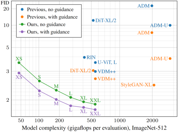
Our recent paper, Analyzing and Improving the Training Dynamics of Diffusion Models, reports the results and details of our research. We meticulously analyze and rethink the training dynamics of the ADM denoiser network, which serves as the basis of many flagship image generator models. We report state-of-the-art performance both in terms of training speed and generation quality for denoising diffusion. As shown in Figure 1, our models reach a comparable quality to prior works, with a fraction of the model complexity and training time, and significantly surpass it with larger models.
We arrived at a streamlined network architecture and training recipe we call EDM2—a robust, clean slate that isolates the powerful core of ADM while shedding the historical baggage and cruft.
Additionally, we shed light on a poorly understood but crucially important procedure of exponential moving averaging of network weights and drastically simplify the tuning of this hyperparameter.
This post explains the key findings of this research. To see the reference implementation code, visit NVlabs/edm2 on GitHub.
What are training dynamics and why do they matter?
Consider the baseline ADM architecture as shown in Figure 2.
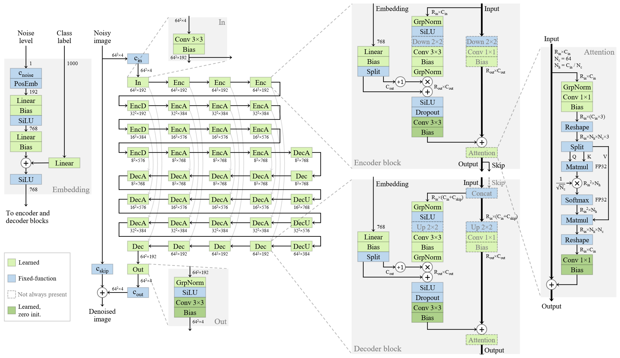
It’s a wonder that we can successfully train such a deep and complex network by bombarding it with a gradient feedback signal sent from the output end. How can we be sure that it actually reaches all parts of the network in a healthy and balanced way and trains each layer to its full potential?
Historically, this was far from clear, and networks would suffer from poor performance due to problems like exploding and vanishing gradients. The situation improved rapidly after introducing modern optimizers and normalization and initialization procedures in the early 2010s. The training dynamics were unblocked, and to this day, we see no end to scaling with model complexity and data.
Liberally sprinkling components like batch or group normalization layers often solves the most glaring issues, and it’s left at that. But are modern networks truly well-oiled learning machines, or are they creaking under the ever-growing complexity of architectures and training tasks? The diffusion loss is extremely noisy and complicated, and on closer inspection, the training is only barely holding things together.
Taking control of weight and activation magnitudes
Here’s the first clue: not everything is right with the training of ADM. Tracking the magnitude of the values seen in the activations propagating in the network and the learned weight tensors stored at the layers shows a steady growth throughout the training (the lines correspond to a selection of different layers).
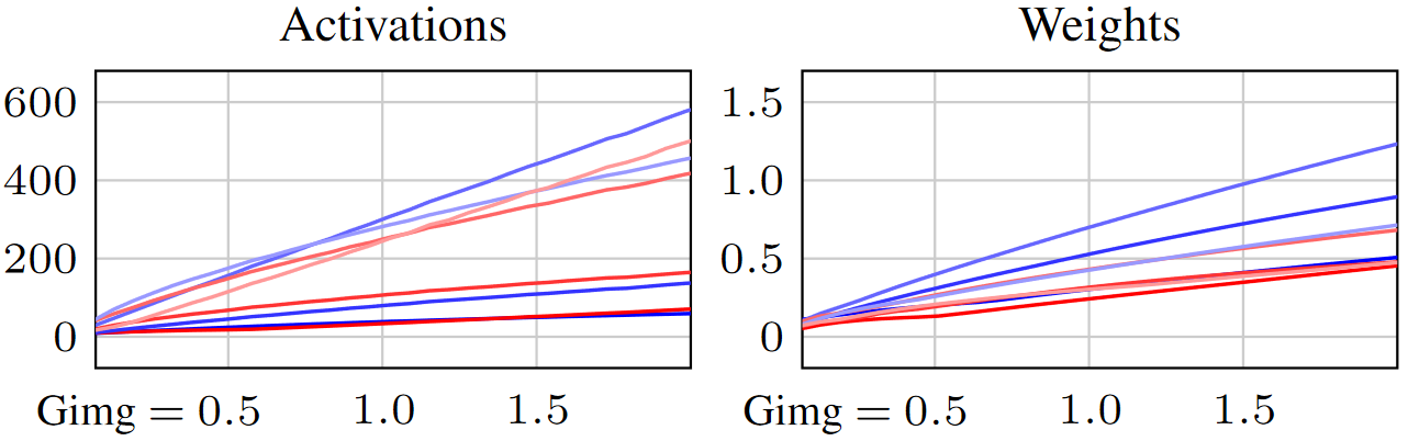
This behavior is common (not just in diffusion) and typically ignored as yet another weird curiosity, as it doesn’t seem to prevent the network from learning. However, we find that this is an unhealthy phenomenon that significantly hampers the speed, reliability, and predictability of the training and compromises the quality of the end result.
Why is this a problem? What causes weight and activation growth, and what harmful effects do they have? These questions open quite a tangle of issues, each feeding into one another in a complex web of interactions.
First, we find that the growth of weights is a numerical artifact and not something the training “knowingly” seeks to do for some beneficial end. It’s a statistical tendency caused by noise and numerical approximation errors in gradient updates. Unfortunately, despite this incidental nature, it’s problematic for two distinct reasons:
- The training gets saturated over time because updates made to the weights make a smaller relative impact when the existing weight is already large. It’s like throwing teaspoons of ingredients into a pot. After a while, adding one more teaspoon doesn’t change much. The training slows down to a crawl—at a different rate at each layer—even when there is more to learn. In other words, the training suffers from uncontrolled per-layer learning rate decay.
- The weights act multiplicatively on the activations through convolutions and matrix products. When a weight grows, so do the activations of that layer. Thus, weight growth causes activation growth.
What about activation growth, then? Why is it a problem?
Viewing the world through the eyes of an individual layer somewhere mid-network, on any training iteration, the input activations it receives have grown slightly larger than it’s used to seeing. Although its weights are adapted to the previously smaller inputs and are therefore out of date, it uses them. Later, it receives a gradient signal that tells it how to fix this discrepancy. But the feedback came too late, and the computation was already slightly wrong. The input activation magnitudes have grown yet again on the next iteration, and the same process repeats.
By induction, under growing activations, all layers are always slightly stale, and the network output is always slightly wrong. No matter how long training continues, the optimum always escapes out of reach. This matters in a high-accuracy task like diffusion denoising.
The remedy
Having recognized the problems, how can they be fixed? To simplify the task, we started by critically examining each moving part in the network and cutting out the unnecessary slack. For example, we removed all learnable biases (surprisingly, with no ill effects), which made it easier to reason about the magnitudes, as it left us with fewer types of learnable parameters. The paper details a number of miscellaneous improvements, which together made the network’s behavior much more predictable and stable.
With this cleaner slate, we proceeded to the core improvements that target the problems detailed previously. The following sections detail the key steps:
- Applying unified magnitude preservation principle for all layers
- Taking control of the effective learning rate
- Dropping the now superseded (and problematic) group normalization layers
Eliminating activation and weight growth
We adopt a simple overarching principle: every layer must preserve the magnitude of its input activations on statistical expectation. With no layer actively changing the activation magnitudes, they remain approximately constant over time and between parts of the network.
We first illustrate this idea with “non-learned” layers like nonlinearities (which we consider separate from the learned layers), concatenations, and additions. For example, a SiLU nonlinearity reduces the magnitude of its input activations, pulling the negative values towards zero. Feeding this layer with a lot of random data, on average, its magnitude would change by a factor of 0.596. The magnitude-preserving version of SiLU divides the output activations by this statistically expected constant, approximately canceling the change in magnitude.
How is this principle applied to convolutions and fully connected layers that contain learnable weights? The expected change in activation magnitude is directly proportional to the weight magnitude. To eliminate this, we rescaled the weights to always remain at unit magnitude (with some subtleties—refer to the paper appendix or the code release for details).
Crucially, this severs the direct causal link where growing weights cause growing activations and eliminates the problem of ever-stale layers. The standardization of activation magnitudes also makes the network more predictable. For example, when combining activations from two distinct branches, we can mix their contributions in a ratio of our choice without one branch accidentally overpowering the other due to uncontrolled magnitudes.
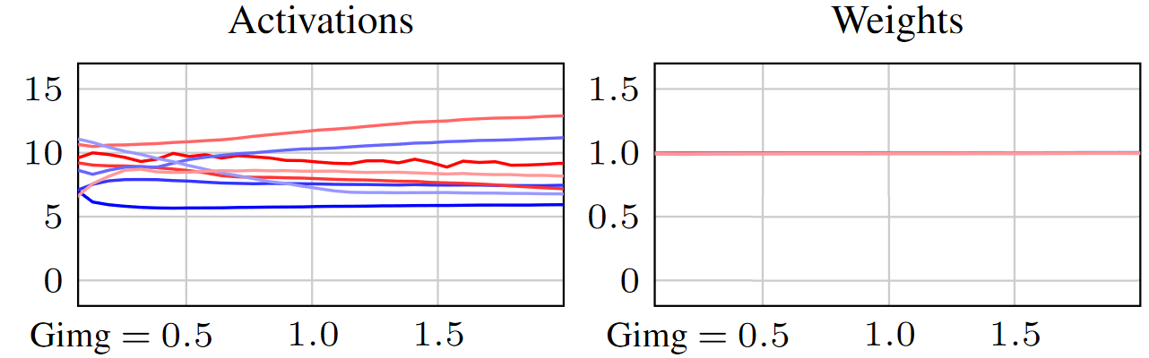
Note how this gets two birds with one stone: the activations remain steady, and the weights are explicitly prevented from growing (Figure 4).
Controlling learning rate decay
Eliminating weight growth also eliminates decay in the uncontrolled learning rate. This is an excellent baseline situation, as each Adam optimizer weight update now has a roughly uniform impact on each weight, regardless of how far the training has progressed or where it’s located within the network.
In contrast, the original network layers had an “effective learning rate” based on their uncontrolled magnitudes: some layers learned too slowly, others so fast as to be unstable; some stopped learning long before they were done, and others never settled down.
However, learning rate decay is necessary, as it allows the network to focus on progressively finer details of the data as it learns. We want to do it on our terms, and under normalized weights, we can trust that all layers follow the specified rate. In practice, simple controlled decay schedules work well in this setting.
Removing group normalization layers
At this point, the numerous group normalization layers in the ADM network have become superfluous, as the magnitude preservation scheme already keeps the activation magnitudes in check. Interestingly, removing them improves the results further. This suggests that direct imposition of activation statistics might have adverse side effects.
This reminded the team of intriguing findings we made some years ago in the original StyleGAN architecture, as detailed in A Style-Based Generator Architecture for Generative Adversarial Networks. It turned out that the generator network had learned to “cheat” by growing a large-magnitude localized blob into its internal activation maps (leaving an ugly mark in the output images). This would bypass the activation magnitude normalization by corrupting the averages it computes. The strict normalization must have seriously limited the network’s aspirations, given the hoops it jumped to escape.
We suspect that dividing out the average magnitude in a given activation tensor introduces inadvertent long-range dependencies and complex balancing requirements among all pixels and features. Weight normalization is gentler in this regard. A bright pixel appearing in one corner doesn’t darken the rest of the image.
Exponential moving averages
Model averaging is a widely used practice in deep learning. The idea is to keep track of a running exponential moving average (EMA) of “recent” weights during training. These weights are not used during the training, but rather at inference time. The thinking is that the raw training weights are noisy and influence the most recently shown training samples too much.
A mystifying aspect of diffusion model training—often hidden in opaque hyperparameter tables in appendices of research papers or default parameters in codebases—is the need to apply a very long average to get good results, often several percent of the entire length of the training. Using the freshest training weights (no EMA) yields disastrously bad results. On the other hand, too much averaging would overemphasize the early-stage weights, including the random initialization. This is inconvenient, as there doesn’t seem to be much logic regarding what rate of averaging works well, and the number needs to be decided before the training. Or does it?
Post-hoc reconstruction
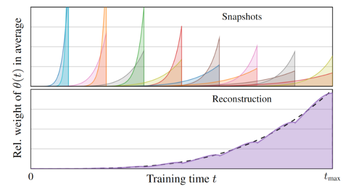
As explained in Analyzing and Improving the Training Dynamics of Diffusion Models, we changed the shape of the EMA profile curve to “stretch” with the length of the training and present a post-hoc method for reconstructing networks with different EMA lengths after the training. The idea is to store periodic snapshots of the intermediate training state with fixed shorter EMA lengths, from which we can later reconstruct a broad range of longer EMA profiles by suitable linear mixtures. Combining a few dozen snapshots is orders of magnitude more efficient than re-running the entire training; determining the optimal EMA length is a straightforward mechanical procedure.
Figure 5 shows an example of how individual snapshots might be combined into a longer average over the weight history. The shaded regions indicate how much of the weights at different times each snapshot collected.
This approach enables plotting performance metrics as a function of the EMA length, giving us unprecedented insight into its behavior. Densely measuring the quality (lower FID score is better) of the generated images as a function of the EMA length (as a percentage of full training run length) gives plots like the one shown in Figure 6. It compares the performance of different network configurations, which are denoted by letters.
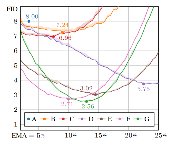
The optimal value is quite sharp, and quality rapidly declines when deviating from it. With the wrong choice of EMA, a good model can show arbitrarily poor performance. Blindly using a suboptimal EMA (say, 8% or 18%) would falsely indicate that the winning configuration G is inferior to some of the other contenders.
Using this new tool uncovers several surprising phenomena. For example, the optimal EMA length is very sensitive to the use of classifier-free guidance (Figure 7).
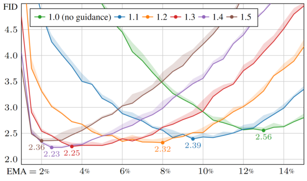
Based on this knowledge, a sweep over EMA values is an essential part of model tuning and evaluation going forward.
Results and conclusions
Our team thoroughly evaluated the improvements in the common ImageNet-512 setting using latent diffusion and reached a record FID of 1.81 in this widely used benchmark. However, simply looking at the bottom line number could be misleading. What matters is the scaling with size.
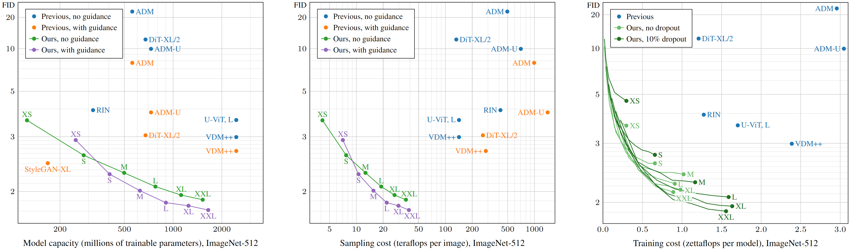
To this end, we trained six increasingly large models called EDM2-XS, S, M, L, XL, and XXL. Figure 1 shows the FID score (quality) as a function of model complexity (gigaflops per evaluation of the network) for each of our models, along with recent state-of-the-art contenders such as diffusion transformers and VDM++. For each model, we also plot a variant with classifier-free guidance enabled during sampling, as this is a crucial tool for improving the results in present diffusion models.
From this, our models uniformly reach the best bang for the buck for a given budget and reach a similar quality as the previous state-of-the-art with a 5x smaller model. Comparisons in terms of parameter count, inference-time sampling expense, and training cost tell a similar story (Figure 8).
Of course, the generated images can and should be looked at, too (Figure 9). But there is a reason why the field relies heavily on metrics, as making visual judgments about the fidelity to training data from a handful of images is difficult.
We also evaluated the performance with the FDDINOv2 metric, which has recently been proposed to improve on some blind spots of FID. We see a similar advantage for our method.
Beyond maximizing performance, one key goal is to simplify the architecture and make it more amenable to tuning and exploration. In our practical experience, the final architecture seems to behave much more predictably, and we find it significantly more robust to changes.
You may have noticed that most of the findings are generic and not tied to the ADM architecture specifically—or even diffusion, for that matter. This is indeed an interesting avenue for future investigation. The principles could also be directly applied to, for example, diffusion transformer training. In prior research, for example, image classifiers have benefited from related redesigns of the normalization schemes. The key components, like forced weight normalization and magnitude-preserving layers, are self-contained and can easily be adopted to other networks.
