Generative AI Research Spotlight: Demystifying Diffusion-Based Models

With Internet-scale data, the computational demands of AI-generated content have grown significantly, with data centers running full steam for weeks or months to train a single model—not to mention the high inference costs in generation, often offered as a service. In this context, suboptimal algorithmic design that sacrifices performance is an expensive mistake.

Much of the recent progress in AI-generated image, video, and audio content has been driven by denoising diffusion—a technique that iteratively shapes random noise into novel samples of the data. A recent research paper published by our team, Elucidating the Design Space of Diffusion Based Models, recipient of the Outstanding Paper Award at NeurIPS 2022, identifies the simple core mechanisms underlying the seemingly complicated approaches in the literature. Starting with this clear view of the fundamentals, we then find the state-of-the-art practices for quality and computational efficiency.

Denoising diffusion 

Denoising is the act of removing, for example, sensor noise from images or hiss from audio recordings. This post will use images as the running example, but the process applies to many other domains as well. This task is excellently suited for convolutional neural networks. 

What does this have to do with generating novel images? Imagine there is a large amount of noise on an image. Indeed, so much that the original image is lost. Could a denoiser be used to reveal some random image that could be hiding under all that noise? Surprisingly, the answer is yes.

This is the simple essence of denoising diffusion: first draw a random image of pure white noise, and then chip away at the noise level—say, 2% at a time—by repeatedly feeding it to a neural denoiser. Gradually, a random clean image emerges from underneath the noise. The distribution of generated content (pictures of cats and dogs? audio waveforms of spoken English phrases? video clips of driving?) is determined by the dataset that the denoiser network was trained with. 

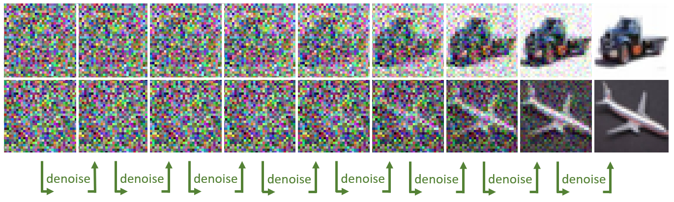
The code below is a first guess of how to implement this idea, assuming a neural network function denoise is available.

# start with an image of pure large-magnitude noise
sigma = 80		# initial noise level
x = sigma * torch.randn(img_shape)

for step in range(256):
    # keep 98% of current noisy image, and mix in 2% of denoising
	x = 0.98 * x + 0.02 * denoise(x, sigma)
	
    # keep track of current noise level
    sigma *= 0.98

If you’ve ever looked at code bases or scientific papers in the field, filled with pages of equations, you might be surprised to learn that this near-trivial piece of code is actually a theoretically valid implementation of something called a probability flow ordinary differential equation solver. While this snippet is hardly optimal, it embodies surprisingly many of the key good practices explained in the paper. The team’s top-of-the-line final sampler is essentially just a few more lines. 

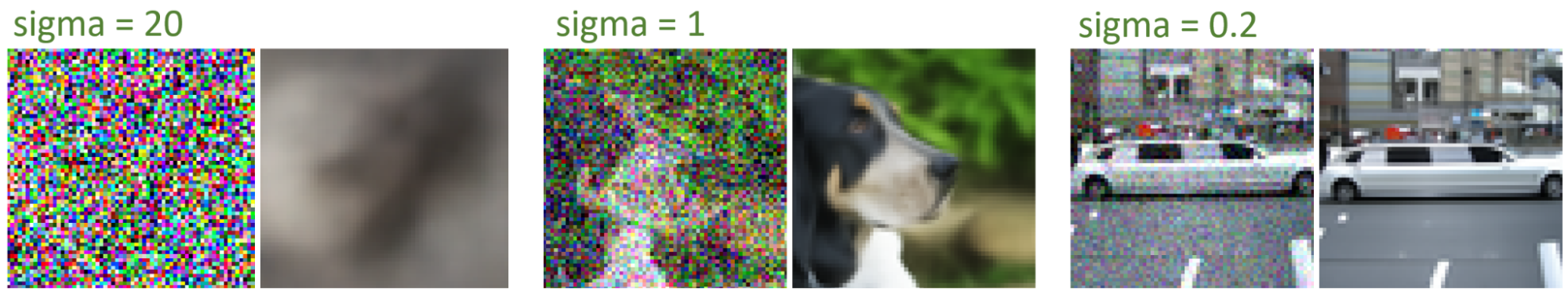
What about that function denoise? At its core, it’s surprisingly straightforward as well: the denoiser must output the blurry average of all possible clean images that could have been hiding under the noise. The desired output at various noise levels might look like the examples in Figure 2.

Training a denoiser network (typically a U-Net) with basic loss—the mean square error between its output and the clean target—achieves precisely this result. Fancier losses that aim for sharper output are in fact harmful, and violate the theory. Keep in mind that, even if the task is conceptually simple, most existing denoisers are not trained for it specifically.

Much of the apparent mathematical complexity in the literature arises from justifying why this works. The theory can be built up from various formalisms, the most popular two being Markov chains and stochastic differential equations. While each approach boils down to a denoising loop that uses a trained denoiser, they open up a vast and confusing space of different practical implementations, and a minefield of opportunities to make poor choices.

The paper peels back the layers of mathematical complexity, directly exposing the tangible design choices in a standardized framework where they are easy to analyze. 

This post presents the team’s key findings and intuitions through visualizations and code. We’ll cover three topics:

• An intuitive overview of the theory behind denoising diffusion
• Design choices related to sampling (generating images when you already have a trained denoiser)
• Design choices when training that denoiser

What makes diffusion work?

To begin, this section takes a step back to the basics and builds the theory that justifies this straightforward piece of code. We find most insight in the differential equation framework, originally presented in Score-Based Generative Modeling through Stochastic Differential Equations. While the equations and mathematical concepts might look intimidating, they are not crucial for understanding the gist. It is useful to mention them occasionally to highlight that they are often just a different language for describing concrete things done in code.

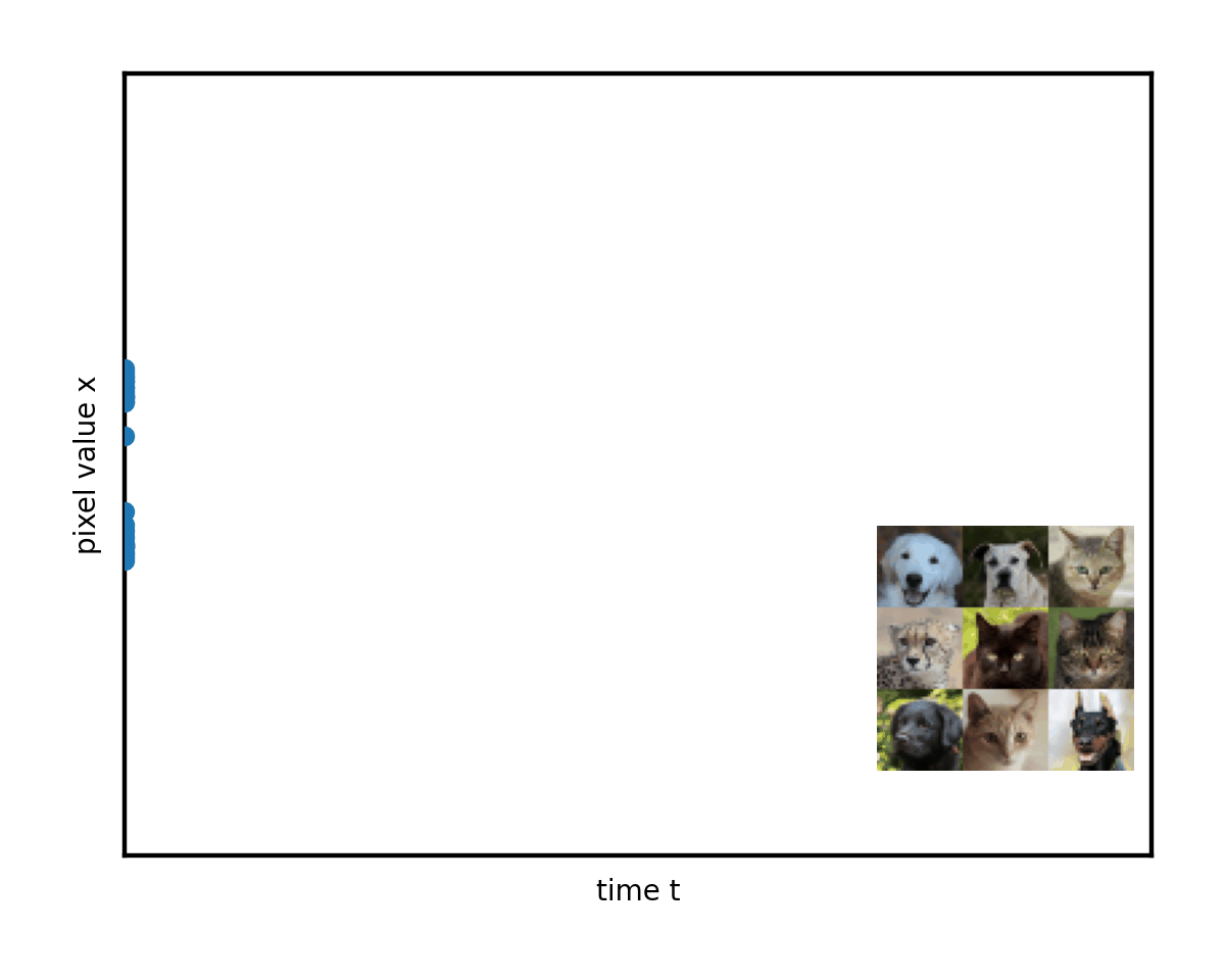
Imagine an RGB image x of shape, say, [3, 64, 64] from the dataset. Begin by considering the easy direction of destroying the image by gradually adding noise onto it. (Of course, this is the opposite of the end goal.)

for step in range(1000):
	x = x + 0.1 * torch.randn_like(x)

This is in fact (suitably squinting) a stochastic differential equation (SDE) solver corresponding to a simple SDE . It says that the change in image x over a short time step is random white noise. Here, solving simply means simulating a specific random numerical realization of the process described by the SDE.

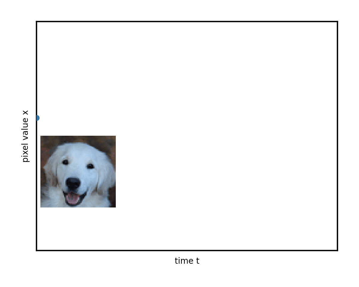
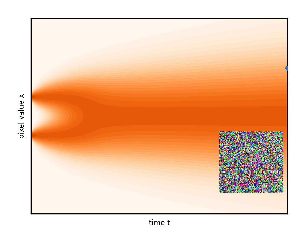
A nice thing about differential equations is that they have a fruitful geometric interpretation. You can visualize this process as the image taking a random walk (the famous Brownian motion, or Wiener process) in the pixel value space. If you consider x above to be just a single number (a “single pixel image”), you can plot its evolution as the following graph. The real thing is exactly the same but in a much higher dimension, so it can’t be visualized on a two-dimensional monitor.

Studying this evolution using many different starting images and random paths, you begin to see some order within the chaos. Think of it like stacking lots of these squiggly paths on top of each other. On average, they create a changing shape over time. 

The complex pattern of data at the left edge (you could metaphorically imagine the two peaks corresponding to images of cats and dogs, respectively) gradually mixes and simplifies into a featureless blob at the right edge. This is the ubiquitous normal distribution, or pure white noise.

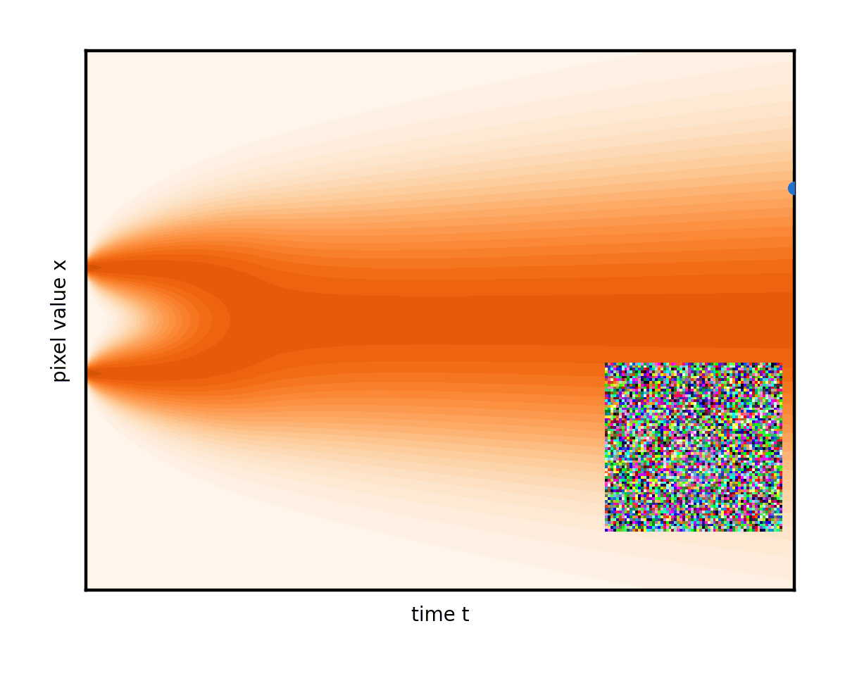
The high-level goal (generative modeling) is to somehow find a trick to sample novel images from the true hidden data distribution on the left in Figure 4—actual new images that could have been in the dataset, but weren’t. You could easily sample from the pure-noise state on the right, using randn. Is it possible to then run the above noising process in the reverse direction, so as to end with random samples of clean images (Figure 5)?

Following a random path starting from the right edge, what guarantees a proper image at the left edge, rather than just more noise? Some kind of additional force is needed to gently pull the image towards the data on each step.

The theory of SDE’s provides a beautiful solution. Without diving too much into the technicalities, it indeed enables reversing the time direction, and doing so automatically introduces an extra term for the sought-after data-attraction force. The force pulls the noisy image towards its mean-square optimal denoising. This can be estimated with a trained neural network (here, sigma is the current noise level):

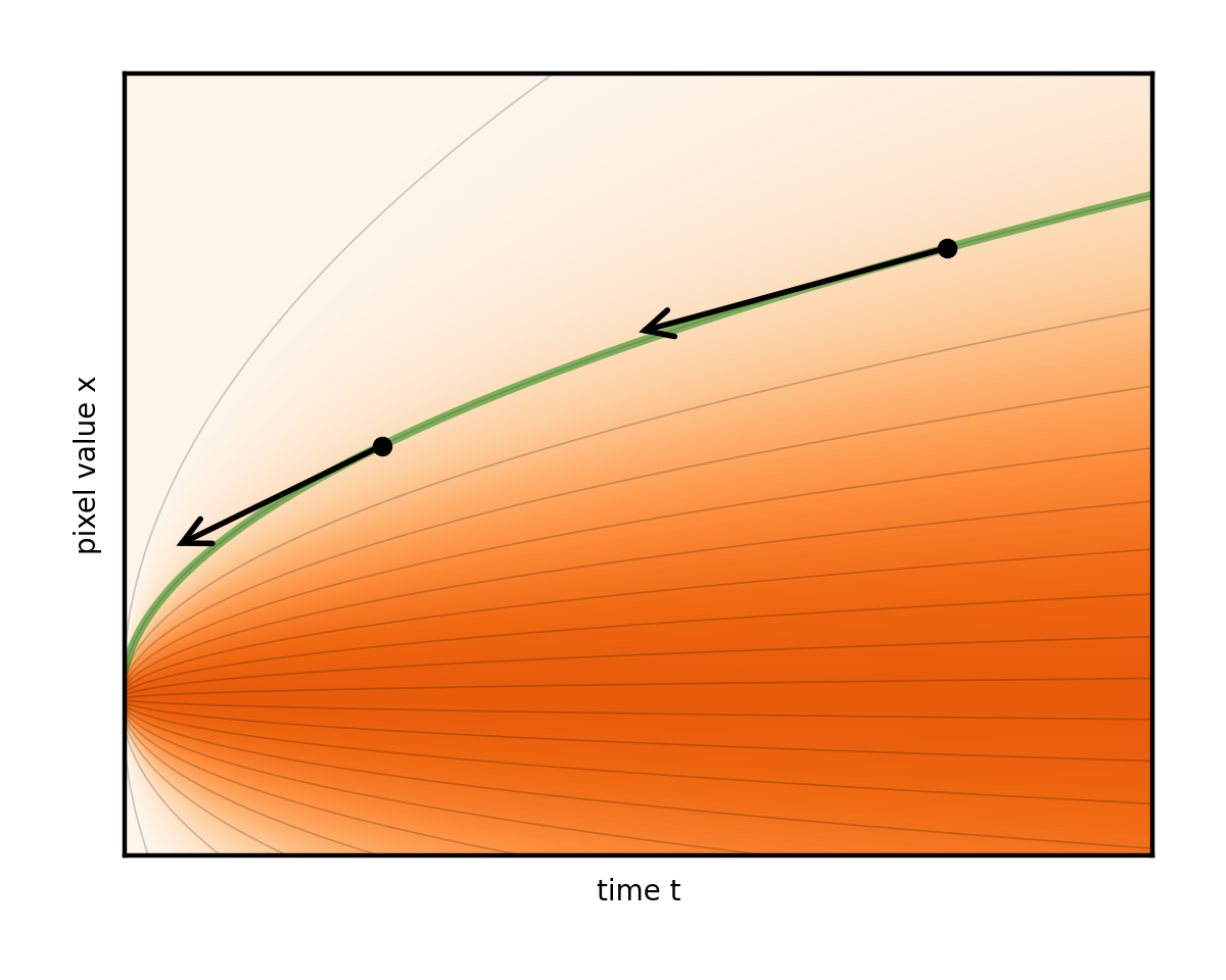
You can even adjust the weight of the two terms, as long as you are careful to keep the total rate of noise reduction unchanged. Taking this idea to the extreme of removing noise exclusively leads to a fully deterministic ordinary differential equation (ODE) with no random component at all. The evolution then follows a smooth trajectory, and the image simply fades in from underneath the fixed noise (Figure 6).

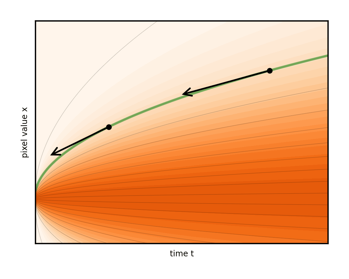
Notice how the curved trajectory in Figure 6 connects the initial random noise at the right edge to a unique generated image at the left edge. Indeed, the ODE establishes a different trajectory for each initial noise. Think of these curves as flow lines of a fluid pushing our image around. During the generation, the task is simply to follow the flow line from the start as accurately as possible. Start from a random spot on the right, and at each step, the formula (really, the denoiser network) shows where the flow line points for the current image. Inch a bit in its direction and repeat. That’s the generation process in a nutshell.

Figure 7 shows that each step of the solver advances the time backward by some chosen amount (dt), and consults the ODE formula (and consequently, the denoiser network) to determine how to change the image over the timestep.

Subsequent sections analyze the deterministic version exclusively, as stochasticity obscures the geometric insight afforded by the deterministic picture. With appropriate tuning, stochasticity has beneficial error correction properties, but it is tedious to use and can be seen as something of a crutch. For more details, see Elucidating the Design Space of Diffusion Based Models.

Design choices for sampling to generate images 

As stated in the introduction, it’s the details that make or break the performance. The key difficulty is that the step direction given by the network is valid only in the immediate vicinity of the current noise level. Trying to reduce too much noise at once without stopping to re-evaluate will result in adding something into the images that shouldn’t be there. This shows up as variously reduced image quality: indescript blobbiness and graininess, color and intensity artifacts, distortions and lack of coherence in faces and other higher-level details, and so on.

In the 1D visualization, this corresponds to taking a step that lands away from the starting flow line, as shown in Figure 8. Notice the gap that opens between the arrows (representing steps that might be taken) and the curve. 

The common brute-force solution is to simply take a large number of very short steps so as to avoid getting thrown off. However, this is expensive because every step incurs a full evaluation of the denoiser network. It’s like crawling instead of running: safe but slow. 

Our sampler design drastically reduces the number of steps required without compromising quality. The strategy is three-fold:

• Design the ODE such that its flow lines are as straight as possible, and hence easy to follow (noise schedules)
• Identify what noise levels still need extra careful stepping (time step discretization)
• Take smarter steps to get the most bang for the buck from each (higher-order solvers)

Straightening the flow for fewer steps

The key issue is the curvature of the flow lines. Had they been straight lines, they would be very easy to follow. It would be possible to take a single long straight step all the way to noise level zero, and never worry about falling off the curve. In reality, some curvature is unavoidably built into the setup. Can it be reduced? 

It turns out that the theory developed in the previous section enables some poor choices in this regard. For example, you can build different versions of the ODE by specifying different noise schedules. Recall that the 1D visualization was built by adding the same amount of noise at each step. Had it been added at some different time-varying rate, each noise level would be reached at some different time (a different schedule). This amounts to stretching and squeezing the time axis. 

Figure 9 shows a few different ODEs that are induced by different noise schedule choices.

Notice that this has the side effect of reshaping the flow lines. In fact, the lines are almost straight in one of these schedules. This is indeed the one that the team advocates. The arrows representing steps now almost perfectly align with the curves. Consequently, it’s possible to take many fewer steps compared to other choices (Figure 10).

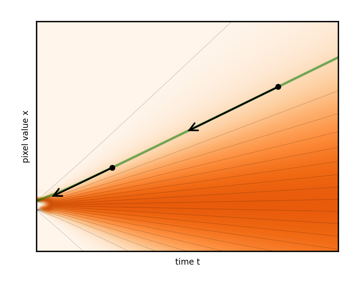
Figure 10 shows a schedule with the noise level growing linearly as time progresses. Contrast the previous example of constant-rate addition, with the noise level growing fast at first but then slowing down. In other words, time becomes synonymous with noise level. Without diving into the technical details here, this particular choice gives the beautifully straightforward solver algorithm. This is Algorithm 1 in our paper, without the optional lines 6 to 8, using the proposed schedule and after some tidying up:

# a (poor) placeholder example time discretization
timesteps = np.linspace(80, 0, num_steps)

# sample an image of random noise at first noise level
x = torch.randn(img_shape) * timesteps[0]

# iterate through pairs of adjacent noise levels
for t_curr, t_next in zip(timesteps[:-1], timesteps[1:]):

    # fraction of noise we keep in this iteration
	blend = t_next / t_curr
	
    # mix in the denoised image
	x = blend * x + (1-blend) * denoise(x, t_curr)

The code is just a slight generalization of the listing in the introduction. It can’t get much simpler than this. The algorithm is so straightforward that one wonders how it wasn’t stumbled upon from heuristic grounds in 2015—perhaps the idea seems too preposterous to work. Incidentally, denoising diffusion was discussed in the 2015 paper, Deep Unsupervised Learning using Nonequilibrium Thermodynamics, but under a complex mathematical guise. Its potential went unnoticed for years. 

Careful stepping at low noise levels

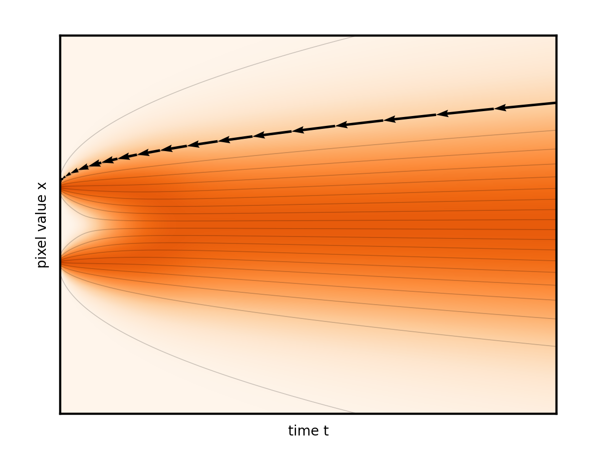
This clearly highlights another design choice, which in most treatments is obscured and entangled with the noise schedule: the choice of time steps. The linear spacing used in the previous code snippet is in fact a poor choice. Empirically (and reasoning from natural image statistics), it’s clear that detail is revealed more rapidly near low noise levels. In the 1D visualization, little is happening for most of the right side of the plot, but then the flow lines take a sudden turn into one of the two basins on the left. This means that long steps are possible at high noise levels, but it is necessary to slow down when approaching low noise levels (Figure 11).

Our paper empirically studies what the relative length of steps should be at low versus high noise levels. The following code snippet arrives at a simple but robust modification for timesteps. Roughly, raise the numbers in it to the power of seven (careful to keep them scaled to the original range of 0 to 80). This strongly biases the steps towards the low noise levels:

sigma_max = 80
sigma_min = 0.002	# leave a microscopic bit of noise for stability
rho = 7

step_indices = torch.arange(num_steps)
timesteps = (sigma_max ** (1 / rho) \
          + step_indices / (num_steps - 1) \
            * (sigma_min ** (1 / rho) - sigma_max ** (1 / rho))) ** rho

Higher-order solvers for more accurate steps

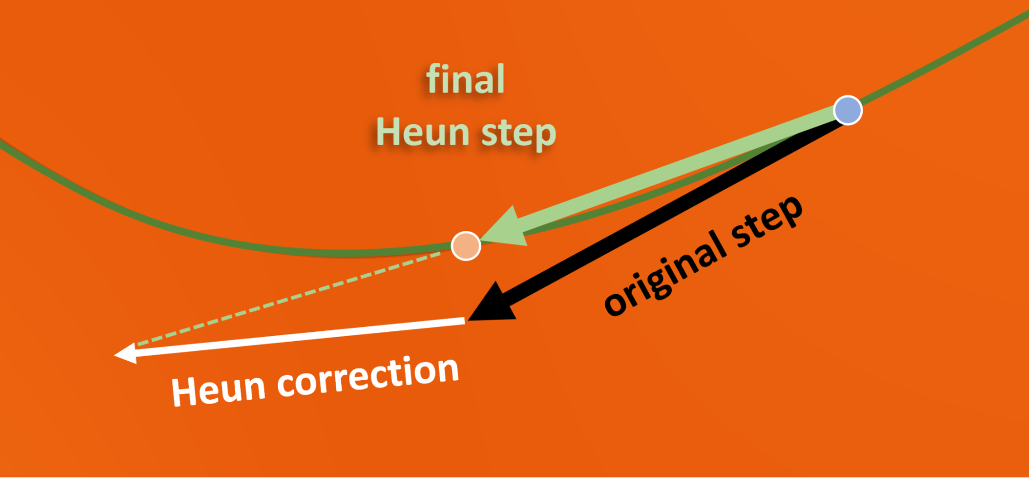
The ODE viewpoint enables the use of fancier higher-order solvers, which essentially take curved instead of linear steps. This is an advantage when trying to follow ‌curved flow lines. The benefits are not clear-cut, as estimating ‌local curvature requires additional neural network evaluations. The team tested a range of approaches and consistently found the so-called second-order Heun scheme to be the best (Figure 12). This adds a couple of lines to the code (see Algorithm 1 in Elucidating the Design Space of Diffusion Based Models) and doubles the expense per iteration, but cuts the number of required iterations to a fraction. 

The Heun step has a nice geometric interpretation and a straightforward implementation in code. Take a tentative step as before, then take a second one, and retrace back halfway from the landing point. Notice how the final corrected step lands much closer to the actual flow line than the original one (Figure 12).

With all of these improvements combined, it now suffices to evaluate the denoiser only 30 to 80 times, as opposed to 250 to 1,000 times as in most previous work.

Design choices for training the denoiser

This is now a sleek and efficient chain of denoising steps. Thus far, it’s been assumed that each step can call a readily-trained denoiser denoise (x, sigma) taking in the noisy image and a number indicating its noise level. But how to‌ parametrize and train it for best results?

The most basic form of theoretically valid training for such a network (here, a PyTorch module instantiated as denoise) would look something like the following:

# WARNING: this code illustrates poor choices across the board!

for clean_image in training_data:	# we’ll ignore minibatching for brevity

	# pick a random noise level to train at
	sigma = np.random.uniform(0, 80)

    # add noise with this level
	noisy_image = clean_image + sigma * torch.randn_like(clean_image)

    # feed to network under training
    denoised_image = denoise(noisy_image, sigma)

    # compute mean square loss
	loss = (denoised_image - clean_image).square().sum()

	# ... plus the usual backpropagation and parameter updates

The theory requires using white noise and mean-square loss, and to touch all the noise levels that are intended for use in sampling. Within these constraints, there is a lot of freedom to rearrange the computations. The following subsections identify and address each of the serious practical problems in this code.

Note that the network architecture itself will not be addressed. This discussion is largely orthogonal and agnostic to layer counts, shapes and sizes, use of attention or transformers, and so on. For all the results in the paper, network architectures from previous work were adopted.

Network-friendly numerical magnitudes

The maximum noise level of 80 in these examples has been empirically chosen as a large enough number to completely drown out the image. Consequently, the denoiser is sometimes fed with an image whose pixel values are roughly in the range of -1 to 1 (when the noise level is very low), and sometimes with images in a range beyond -100 to 100. This raises a red flag, as neural networks are known to suffer from unstable training and poor final performance if their inputs vary vastly in scale between examples. It is necessary to standardize the scales.

Some works combat this by modifying the ODE itself, such that the sampling process keeps the noisy image in a constant-magnitude range rather than allowing it to expand over time (a so-called variance preserving scale schedule). Unfortunately, this distorts the flow lines again, defeating the benefits of straightening uncovered in the previous section.

A straightforward solution that does not suffer from such numerical drawbacks follows. The noise level is known, so simply scale the noisy image to a standard magnitude before feeding it to the network. It will automatically adapt to the different scale convention through training, but the problematic range variation is eliminated. 

The clean way to achieve this is to keep denoise unchanged from the viewpoint of external callers (the ODE solver and the training loop), but change the way it utilizes the network internally. Isolate the actual raw network layers into their own black box module net, and wrap it with magnitude management code (“preconditioning”) within denoise:

sigma_data = 0.5	# approximate standard deviation of ImageNet pixels
def denoise(noisy_image, sigma):
    noisy_image_variance = sigma**2 + sigma_data**2
	scaled_noisy_image = noisy_image / noisy_image_variance ** 0.5
	return net(scaled_noisy_image, sigma)

Here, the noisy image is divided by its expected standard deviation to bring it roughly to unit variance.

As a minor detail (not shown here), similarly also warp the noise level label input to net with a logarithmic function to make it more evenly spread around the range of -1 to 1.

Predicting the image versus the noise

If you’re familiar with existing diffusion methods, you may have noticed that most of them train the network to predict noise (in unit variance) instead of the clean image, explicitly scale it to the known noise level sigma, and then recover the denoised image by subtraction from input. 

It turns out that this is a good idea specifically at low noise levels, but a bad one at high noise levels. Because most image detail is suddenly revealed at relatively low noise levels, the benefits outweigh the drawbacks.

Why is this a good idea at low noise levels? This approach recycles the almost-clean image from the input, and only uses the network to add a small noise correction to it. Importantly, the network output is explicitly scaled down (by sigma) to match the noise level. Consequently, if the network makes some error (as it always does), that error becomes downscaled as well, and has less of an opportunity to mess up the image. This minimizes the contribution from the unreliable learned network, and maximizes the re-use of what is already known in the input.

Why is this a bad idea at high noise levels? It ends up boosting the network output according to the large noise magnitude. Consequently, any small error the network makes now becomes a big error in the denoiser output.

A better option is a continuous transition, where the network‌ predicts a noise level dependent mixture of the (negative) noise and clean image. Then blend this with the noisy input in appropriate quantities to cancel the noise out.

The paper presents a principled way to calculate the blending weights as a function of the noise level. The exact statistical argument is somewhat involved, so this post won’t attempt to replicate it in full. Basically, it is asking for the blend coefficients that result in minimal amplification of the network output. The implementation is quite straightforward. The last return line is replaced with the code below, where c_skip and c_out are those blend factors controlling how much of the input is recycled, and how much the network contributes, respectively.

return c_skip * noisy_image + c_out * net(scaled_noisy_image, sigma)

Equalizing the gradient feedback magnitudes across noise levels

With the denoiser internals done, this section addresses the noise level issues in our straw-man training code snippet. It was a (poor) implicit choice not to apply any noise-level-dependent scaling on the loss. It’s as though the following was written:

weight = 1
loss = weight * (denoised_image - clean_image).square().sum()

The problem is that the value of this loss is large for some noise levels and small for others, due to the various scalings inside the denoiser. Consequently, the magnitude of the updates (gradient feedback) made to the network weights will also depend on the noise level. It’s like a different learning rate was used for different noise levels, for no good reason. 

This is yet another situation where unifying the magnitudes leads to a more stable and successful training. Fortunately, a simple data-independent statistical formula gives the expected loss magnitude for each noise level. weight is set accordingly to scale this magnitude back to 1.

Allocating ‌training efforts

A tempting misuse of weight could be also weighing the noise levels according to their relative importance, so as to direct more network capacity where it counts. However, the same goal can be achieved without impacting the magnitudes by training more often at those important noise levels. The division of labor the team advocates is conceptually illustrated in Figure 13. 

Each noise level contributes gradient updates (the arrows) to the network weights throughout the training. Separately, we took control of the magnitudes and counts of these updates using the two respective mechanisms. By default, both the magnitude (length of the arrows) and the frequency (their number) depends on the noise level in an uncontrolled manner. The team advocates a division of labor where the loss scaling standardizes the lengths, and noise level distribution decides how often to train at each level.

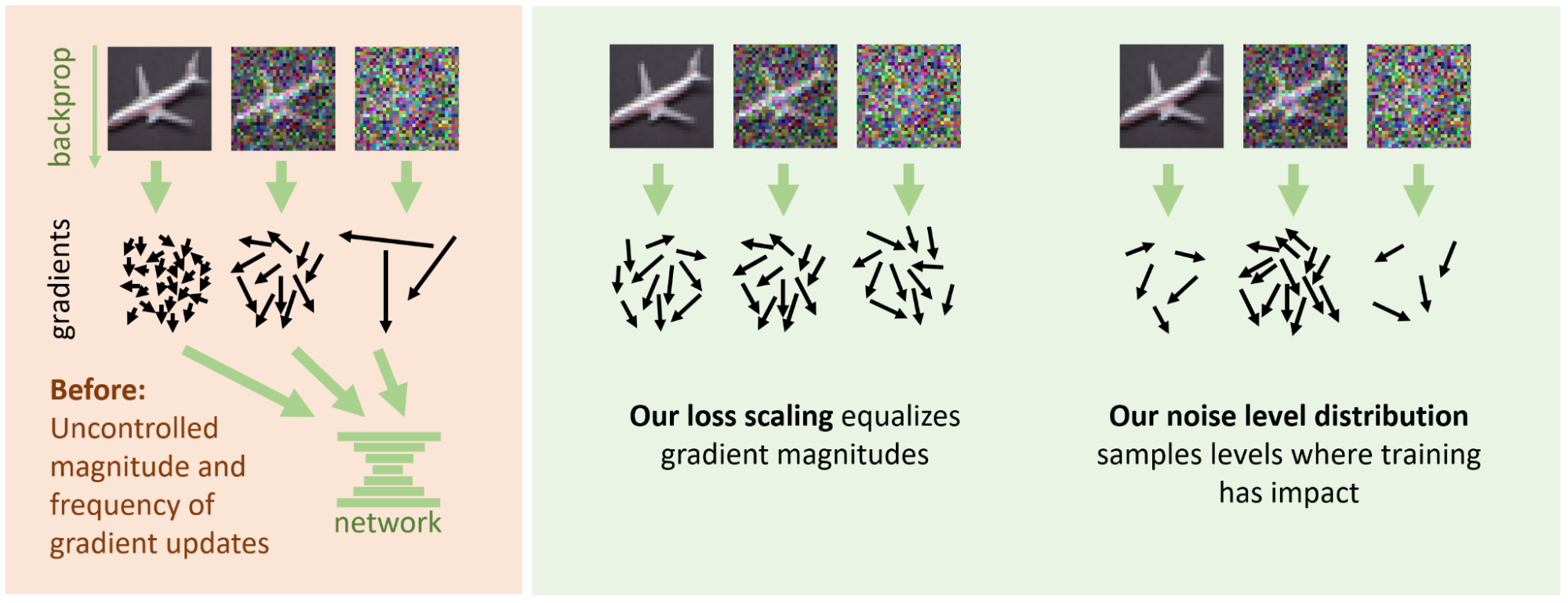
Unsurprisingly, the code example that selects the training noise level from a uniform distribution is a poor choice. The theory offers quite little guidance in this choice, as it depends on the characteristics of the dataset. At very low noise levels, progress is minimal because predicting the noise from a noise-free image is effectively impossible (but also irrelevant). Conversely, at very high noise levels, the optimal denoising (blurry average of dataset images) is rather easy to predict. The middle provides a broad range of levels where progress can be made. 

In practice, we chose the random training noise levels from the formula sigma = torch.exp(P_mean + P_std * torch.randn([])), where P_mean and P_std specify the average noise level for training, and the breadth of randomization around that value, respectively. This specific formula was chosen simply because it’s a straightforward heuristic for drawing non-negative random values spanning multiple orders of magnitude. The values for these parameters are tuned empirically, but turn out to be fairly robust across regular image datasets.

To summarize, below is a minimal piece that brings together all the discussed changes to our original training code, including any omitted formulas: 

P_mean = -1.2		# average noise level (logarithmic)
P_std = 1.2		# spread of random noise levels
sigma_data = 0.5	# ImageNet standard deviation

def denoise(noisy_image, sigma):
	    # Input, output and skip scale
    	c_in = 1 / torch.sqrt(sigma_data**2 + sigma**2)
    	c_out = sigma * sigma_data / torch.sqrt(sigma**2 + sigma_data**2)
    	c_skip = sigma_data**2 / (sigma**2 + sigma_data**2)
    	c_noise = torch.log(sigma) / 4		# noise label warp

	    # mix the input and network output to extract the clean image
        return c_skip * noisy_image + \
                   c_out  * net(c_in * noisy_image, c_noise)

for clean_image in training_data:	# we’ll ignore minibatching for brevity
       # random noise level
        sigma = torch.exp(P_mean + P_std * torch.randn([]))

       noisy_image = clean_image \
                            + sigma * torch.randn_like(clean_image)
       denoised_image = denoise(noisy_image, sigma)
	
	   # weighted least squares loss
       weight = (sigma**2 + sigma_data**2) / (sigma * sigma_data)**2
	   loss = weight * (denoised_image - clean_image).square().sum()

	   # ... plus backpropagation and optimizer update

Results and conclusions

All findings presented in this post are shown to be beneficial by thorough numerical experiments, as detailed in Elucidating the Design Space of Diffusion Based Models. The net effect of incorporating all the improvements is a significant advancement of previous work. In particular, we held the world record FID metric in the highly competitive Imagenet 64×64 category for some while. Moreover, we achieved this record with a greatly reduced number of denoiser evaluations at generation time.

We believe these findings remain relevant into the future with other data modalities, improved network architectures, or higher-resolution images. Of course, one should still be mindful of the underlying reasoning when applying the model in a different context. For example, many constants (such as that maximum noise level of 80, or position and width of the training noise level distribution) will surely need to be adjusted when, for example, adopting latent diffusion or raising the resolution.

To see our official implementation along with pretrained networks, visit NVlabs/edm on GitHub. The code is a clean and minimal implementation that follows the paper notation and conventions, and could serve as an excellent starting point for experimenting and building on these ideas. Note that we include several functions and classes that reproduce previous methods for comparison, but these are not required to use or study our method. For the particularly relevant code, see:

• generate.py
  • edm_sampler implements the full sampler, including optional stochasticity
• training/
  • loss.EDMLoss for the loss function and weightings
  • networks.EDMPrecond for the scale management and mixture prediction
  • networks.DhariwalUNet for our reimplementation of the commonly used ADM network architecture

The team has also just recently published a follow-up research paper, Analyzing and Improving the Training Dynamics of Diffusion Models that picks up where this post ends. In this work, they achieve record-breaking generation quality through a deep dive into the design and training of the denoiser network.