Improving Diffusion Models as an Alternative To GANs, Part 2

This is part of a series on how researchers at NVIDIA have developed methods to improve and accelerate sampling from diffusion models, a novel and powerful class of generative models. Part 1 introduced diffusion models as a powerful class for deep generative models and examined their trade-offs in addressing the generative learning trilemma.

While diffusion models satisfy both the first and second requirements of the generative learning trilemma, namely high sample quality aand diversity, they lack the sampling speed of traditional GANs. In this post, we review three recent techniques developed at NVIDIA for overcoming the slow sampling challenge in diffusion models.

Latent space diffusion models

One of the main reasons why sampling from diffusion models is slow is that mapping from a simple Gaussian noise distribution to a challenging multimodal data distribution is complex. Recently, NVIDIA introduced the Latent Score-based Generative Model (LSGM), a new framework that trains diffusion models in a latent space rather than the data space directly.

In LSGM, we leverage a variational autoencoder (VAE) framework to map the input data to a latent space and apply the diffusion model there. The diffusion model is then tasked with modeling the distribution over the latent embeddings of the data set, which is intrinsically simpler than the data distribution.

Novel data synthesis is achieved by first generating embeddings through drawing from a simple base distribution followed by iterative denoising, and then transforming this embedding using a decoder to data space (Figure 1).

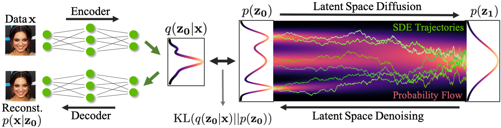
The data and latent spaces are mapped to each other using autoencoders. A diffusion model is formed on the latent encoding of the data. — *Figure 1. Latent score-based generative model*

Figure 1 shows that in the latent score-based generative model (LSGM):

Data $\bf{x}$ is mapped to latent space through an encoder $q(\bf{z}_0|\bf{x})$ .
A diffusion process is applied in the latent space $(\bf{z}_0 \rightarrow \bf{z}_1)$ .
Synthesis starts from the base distribution $p(\bf{z}_1)$ .
It generates samples $\bf{z}_0$ in latent space through denoising $(\bf{z}_0 \leftarrow \bf{z}_1)$ .
The samples are mapped from latent to data space using a decoder $p(\bf{x}|\bf{z}_0)$ .

LSGM has several key advantages: synthesis speed, expressivity, and tailored encoders and decoders.

Synthesis speed

By pretraining the VAE with a Gaussian prior first, you can bring the latent encodings of the data distribution close to the Gaussian prior distribution, which is also the diffusion model’s base distribution. The diffusion model only has to model the remaining mismatch, resulting in a much less complex model from which sampling becomes easier and faster.

The latent space can be tailored accordingly. For example, we can use hierarchical latent variables and apply the diffusion model only over a subset of them or at a small resolution, further improving synthesis speed.

Expressivity

Training a regular diffusion model can be considered as training a neural ODE directly on the data. However, previous works found that augmenting neural ODEs, as well as other types of generative models, with latent variables often improves their expressivity.

We expect similar expressivity gains from combining diffusion models with a latent variable framework.

Tailored encoders and decoders

As you use the diffusion model in latent space, you can use carefully designed encoders and decoders mapping between latent and data space, further improving synthesis quality. The LSGM method can therefore be naturally applied to noncontinuous data.

In principle, LSGM can easily model data such as text, graphs, and similar discrete or categorical data types by using encoder and decoder networks that transform this data into continuous latent representations and back.

Regular diffusion models that operate on the data directly could not easily model such data types. The standard diffusion framework is only well defined for continuous data, which can be gradually perturbed and generated in a meaningful manner.

Results

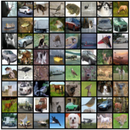
Experimentally, LSGM achieves state-of-the-art Fréchet inception distance (FID), a standard metric to quantify visual image quality, on CIFAR-10 and CelebA-HQ-256, two widely used image generation benchmark data sets. On those data sets, it outperforms prior generative models, including GANs.

On CelebA-HQ-256, LSGM achieves a synthesis speed that is faster than previous diffusion models by two orders of magnitude. LSGM requires only 23 neural network calls when modeling the CelebA-HQ-256 data, compared to previous diffusion models trained on the data space that often rely on hundreds or thousands of network calls.

Video 1. Sequence generated by randomly traversing the latent space of LSGM

Critically damped Langevin diffusion

A crucial ingredient in diffusion models is the fixed forward diffusion process to gradually perturb the data. Together with the data itself, it uniquely determines the difficulty of learning the denoising model. Hence, can we design a forward diffusion that is particularly easy to denoise and therefore leads to faster and higher-quality synthesis?

Diffusion processes like the ones employed in diffusion models are well studied in areas such as statistics and physics, where they are important in various sampling applications. Taking inspiration from these fields, we recently proposed critically damped Langevin diffusion (CLD).

In CLD, the data that must be perturbed are coupled to auxiliary variables that can be considered velocities, similar to velocities in physics in that they essentially describe how fast the data moves towards the diffusion model’s base distribution.

Like a ball that is dropped on top of a hill and quickly rolls into a valley on a relatively direct path accumulating a certain velocity, this physics-inspired technique helps the data to diffuse quickly and smoothly. The forward diffusion SDE that describes CLD is as follows:

$\dbinom{d \bf{x}_t}{d \bf{v}_t} = \underbrace{ \dbinom{M^{1} \bf{v}_t}{\bf{x} t} \beta dt}_{\textrm{Hamiltonian~component} =: \it{H}} + \underbrace{ \dbinom{ \bf{0} d}{-\Gamma M^{-1}\bf{v}_t} \beta dt + \dbinom{0}{\sqrt{2 \Gamma \beta}} d \bf{w}_t}_{\textrm{Ornstein-Uhlenbeck~process} =: \it{O}}$

Here, $\bf{x}_t$ denotes the data and $\bf{v}_t$ the velocities. $M$ , $\Gamma$ , and $\beta$ are parameters that determine the diffusion as well as the coupling between velocities and data. $d\bf{w}_t$ is a Gaussian white noise process, responsible for noise injection, as seen in the formula.

CLD can be interpreted as a combination of two different terms. First is an Ornstein-Uhlenback process, the particular kind of noise injection process used here, which acts on the velocity variables $\bf{v}_t$ .

Second, the data and velocities are coupled to each other as in Hamiltonian dynamics, such that the noise injected into the velocities also affects the data $\bf{x}_t$ . Hamiltonian dynamics provides a fundamental description of the mechanics of physical systems, like the ball rolling down a hill from the example mentioned earlier.

Figure 2 shows how data and velocity diffuse in CLD for a simple one-dimensional toy problem:

Visualization of critically-damped Langevin diffusion run in the joint data-velocity space using 1D toy distributions. — Figure 2. In critically-damped Langevin diffusion, the data x_t is augmented with a velocity v_t. A diffusion coupling x_t and v_tis run in the joint data-velocity space (probabilities in red). Noise is injected only into v_t. This leads to smooth diffusion trajectories (green) for the data x_t.

At the beginning of the diffusion, we draw a random velocity from a simple Gaussian distribution and the full diffusion then takes place in the joint data-velocity space. When looking at the evolution of the data (lower right in the figure), the model diffuses in a significantly smoother manner than for previous diffusions.

Intuitively, this should also make it easier to denoise and invert the process for generation. We obtain this behavior only for a particular choice of the diffusion parameters $M$ and $\Gamma$ , specifically for $\Gamma^2 = 4M$ . This configuration is known as critical damping in physics and corresponds to a special case of a broader class of stochastic dynamical systems known as Langevin dynamics—hence the name critically damped Langevin diffusion.

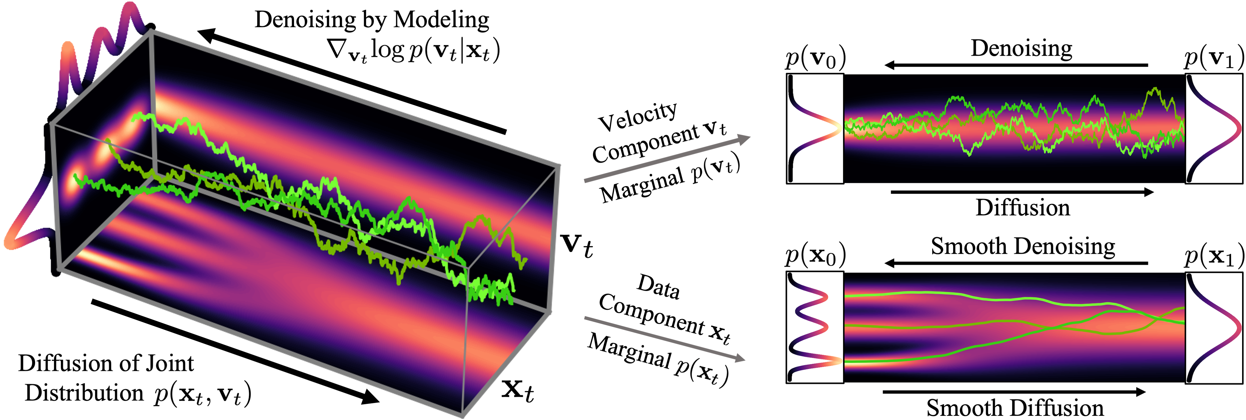
We can also visualize how images evolve in the high-dimensional joint data-velocity space, both during forward diffusion and generation:

Animation of critically-damped Langevin diffusion’s forward diffusion and reverse-time synthesis processes. — Figure 3. CLD’s forward diffusion and the reverse-time synthesis processes

At the top of Figure 3, we visualize how a one-dimensional data distribution together with the velocity diffuses in the joint data-velocity space and how generation proceeds in the reverse direction. We sample three different diffusion trajectories and also show the projections into data and velocity space on the right. At the bottom, we visualize a corresponding diffusion and synthesis process for image generation. We see that the velocities “encode” the data at intermediate times $t$ .

Using CLD when training generative diffusion models leads to two key advantages:

Simpler score function and training objective
Accelerated sampling with tailored SDE solvers

Simpler score function and training objective

In regular diffusion models, the neural network is tasked with learning the score function $\nabla_{\bf {x}t} log ~p_t (\bf{x}_t)$ of the diffused data distribution. In CLD-based models, in contrast, we are tasked with learning $\nabla{\bf {v}_t} log ~p_t (\bf{v}_t|\bf{x}_t)$ , the conditional score function of the velocity given the data. This is a consequence of injecting noise only into the velocity variables.

However, as the velocity always follows a smoother distribution than the data itself, this is an easier learning problem. The neural networks used in CLD-based diffusion models can be simpler, while still achieving high generative performance. Related to that, we can also formulate an improved and more stable training objective tailored to CLD-based diffusion models.

Accelerated sampling with tailored SDE solvers

To integrate CLD’s reverse-time synthesis SDE, you can derive tailored SDE solvers for more efficient denoising of the smoother forward diffusion arising in CLD. This results in accelerated synthesis.

Experimentally, for the widely used CIFAR-10 image modeling benchmark, CLD outperforms previous diffusion models in synthesis quality for similar neural network architectures and sampling compute budgets. Furthermore, CLD’s tailored SDE solver for the generative SDE significantly outperforms solvers such as Euler–Maruyama, a popular method to solve the SDEs arising in diffusion models, in generation speed. For more information, see Score-Based Generative Modeling with Critically-Damped Langevin Diffusion.

CIFAR-10 images generated by a diffusion model based on critically-damped Langevin diffusion. — *Figure 4. Synthesized CIFAR-10 images generated by a diffusion model based on critically damped Langevin diffusion.*

We’ve shown that you can improve diffusion models by merely designing their fixed forward diffusion process in a careful manner.

Denoising diffusion GANs

So far, we’ve discussed how to accelerate sampling from diffusion models by moving the training data to a smooth latent space as in LSGM or by augmenting the data with auxiliary velocity variables and designing an improved forward diffusion process as in CLD-based diffusion models.

However, one of the most intuitive ways to accelerate sampling from diffusion models is to directly reduce the number of denoising steps in the reverse process. In this part, we go back to discrete-time diffusion models, trained in the data space and analyze how the denoising process behaves as you reduce the number of denoising steps and perform large steps.

In a recent study, we observed that diffusion models commonly assume that the learned denoising distributions $p_{ \theta} (\bf{x}_{t-1}|\bf{x}_t)$ in the reverse synthesis process can be approximated by Gaussian distributions. However, it is known that the Gaussian assumption holds only in the infinitesimal limit of many small denoising steps, which ultimately leads to the slow synthesis of diffusion models.

When the reverse generative process uses larger step sizes (has fewer denoising steps), we need a non-Gaussian, multimodal distribution for modeling the denoising distribution $p_{ \theta} (\bf{x}_{t-1}|\bf{x}_t)$ .

Intuitively, in image synthesis, the multimodal distribution arises from the fact that multiple plausible and clean images may correspond to the same noisy image. Because of this multimodality, simply reducing the number of denoising steps, while keeping the Gaussian assumption in the denoising distributions, hurts generation quality.

Visualization of diffused 1D data distributions in diffusion models and of the true denoising distributions for different step sizes during denoising. — *Figure 5.* (top) Evolution of a 1D data distribution q(x₀) according to the forward diffusion process. (bottom) *Visualizations of the true denoising distribution when conditioning on a fixed x₅ with varying step sizes shown in different colors.*

In Figure 5, the true denoising distribution for a small step size (shown in yellow) is close to a Gaussian distribution. However, it becomes more complex and multimodal as the step size increases.

Inspired by the preceding observation, we propose to parametrize the denoising distribution with an expressive multimodal distribution to enable denoising with large steps. In particular, we introduce a novel generative model, Denoising Diffusion GAN, in which the denoising distributions are modeled with conditional GANs (Figure 6).

Visualization of the generative denoising process in diffusion models with Gaussian denoising distributions and with Denoising Diffusion GAN. — *Figure 6. Denoising diffusion process*

Generative denoising diffusion models typically assume that the denoising distribution can be modeled by a Gaussian distribution. This assumption holds only for small denoising steps, which in practice translates to thousands of denoising steps in the synthesis process.

In our Denoising Diffusion GANs, we represent the denoising model using multimodal and complex conditional GANs, enabling us to efficiently generate data in as few as two steps.

Denoising Diffusion GANs are trained using an adversarial training setup (Figure 7). Given a training image $\bf{x}_0$ , we use the forward Gaussian diffusion process to sample from both $\bf{x}_{t-1}$ and $\bf{x}_t$ , the diffused samples at two successive steps.

Given $\bf{x}_t$ , our conditional denoising GAN first stochastically generates $\bf{x}'_0$ and then uses the tractable posterior distribution $q(\bf{x}'_{t-1}|\bf{x}_t, \bf{x}'_0)$ to generate $\bf{x}'_{t-1}$ by adding back noise. A discriminator is trained to distinguish between the real $(\bf{x}_{t-1}, \bf{x}_t)$ and the generated $(\bf{x}'_{t-1}, \bf{x}_t)$ pairs and provides feedback to learn the conditional denoising GAN.

After training, we generate novel instances by sampling from noise and iteratively denoising it in a few steps using our Denoising Diffusion GAN generator.

Schematic visualization of the training pipeline of Denoising Diffusion GAN. — *Figure 7. Training process of Denoising Diffusion GAN*s

We train a conditional GAN generator to denoise inputs $x_t$ using an adversarial loss for different steps in the diffusion process.

Advantages over traditional GANs

Why not just train a GAN that can generate samples in one shot using a traditional setup, in contrast to our model that iteratively generates samples by denoising? Our model has several advantages over traditional GANs.

GANs are known to suffer from training instabilities and mode collapse. Some possible reasons include the difficulty of directly generating samples from a complex distribution in one shot, as well as overfitting problems when the discriminator only looks at clean samples.

In contrast, our model breaks the generation process into several conditional denoising diffusion steps in which each step is relatively simple to model, due to the strong conditioning on $x_t$ . The diffusion process smoothens the data distribution, making the discriminator less likely to overfit.

We observe that our model exhibits better training stability and mode coverage. In image generation, we observe that our model achieves sample quality and mode coverage competitive with diffusion models while requiring only as few as two denoising steps. It achieves up to 2,000x speed-up in sampling compared to regular diffusion models. We also find that our model significantly outperforms state-of-the-art traditional GANs in sample diversity, while being competitive in sample fidelity.

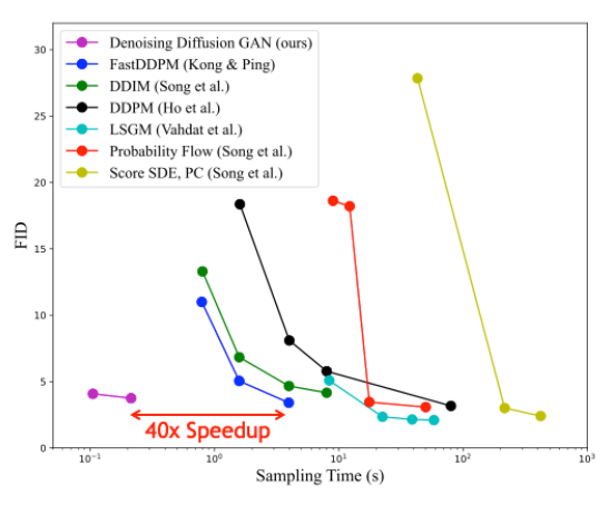
Plot of sample quality vs. sampling time for different denoising diffusion-based generative models. — *Figure 8. Sample quality vs. sampling time for different diffusion-based generative models*

Figure 8 shows sample quality (as measured by Fréchet inception distance; lower is better) compared to sampling time for different diffusion-based generative models for the CIFAR-10 image modeling benchmark. Denoising Diffusion GANs achieve a speedup of several orders of magnitude compared to other diffusion models while maintaining similar synthesis quality.

Conclusion

Diffusion models are a promising class of deep generative models due to their combination of high-quality synthesis and strong diversity and mode coverage. This is in contrast to methods such as regular GANs, which are popular but often suffer from limited sample diversity. The main drawback of diffusion models is their slow synthesis speed.

In this post, we presented three recent techniques developed at NVIDIA that successfully address this challenge. Interestingly, they each approach the problem from different perspectives, analyzing the different components of diffusion models:

Latent space diffusion models essentially simplify the data itself, by first embedding it into a smooth latent space, where a more efficient diffusion model can be trained.
Critically damped Langevin diffusion is an improved forward diffusion process that is particularly well suited for easier and faster denoising and generation.
Denoising diffusion GANs directly learn a significantly accelerated reverse denoising process through expressive multimodal denoising distributions.

We believe that diffusion models are uniquely well-suited for overcoming the generative learning trilemma, in particular when using techniques like the ones highlighted in this post. These techniques can also be combined, in principle.

In fact, diffusion models have already led to significant progress in deep generative learning. We anticipate that they will likely find practical use in areas such as image and video processing, 3D content generation and digital artistry, and speech and language modeling. They will also find use in fields such as drug discovery and material design, as well as various other important applications. We think that diffusion-based approaches have the potential to power the next generation of leading generative models.

Last but not least, we are part of the organizing committee for a tutorial on diffusion models, their foundations, and applications, held in conjunction with the Computer Vision and Pattern Recognition (CVPR) conference, on June 19, 2022, in New Orleans, Louisiana, USA. If you are interested in this topic, we invite you to see our Denoising Diffusion-based Generative Modeling: Foundations and Applications tutorial.

To learn more about the research that NVIDIA is advancing, see NVIDIA Research.

For more information about diffusion models, see the following resources:

Score-based Generative Modeling in Latent Space paper
- Project page: /LSGM GitHub repo
Score-Based Generative Modeling with Critically-Damped Langevin Diffusion paper
- Project page: /CLD-SGM GitHub repo
Tackling the Generative Learning Trilemma with Denoising Diffusion GANs paper
- Project page: /denoising-diffusion-gan GitHub repo

Improving Diffusion Models as an Alternative To GANs, Part 2