Machine learning (ML) can extract deep, complex insights out of data to help make decisions. In many cases, using more advanced models delivers real business value through significantly improving on traditional regression models. Unfortunately, using traditional infrastructure to explain what drove a particular decision with a more advanced model can be difficult, time-consuming, and expensive.
To be confident in the results, we must address explainability. Existing techniques can be slow and are compute expensive—ideal candidates for GPU acceleration. By moving to GPU-accelerated models and explainability, you can improve processing, accuracy, explainability, and provide results when your business needs them.
In this post, we demonstrate how to use advanced models and, with GPU acceleration, allow for the easy, cost-effective, and understandable application of model explainability. We do this in the context of an important business problem, predicting mortgage delinquencies, using a public dataset. This same example could be extended to mortgage or credit underwriting, mortgage prepayment analytics, credit card delinquency, or a host of other important problems.
Classifying mortgage loans
Mortgage lenders are understandably deeply interested in whether they will be paid back in a timely fashion. When delinquency occurs, such as a 90-day past due loan event, concern is raised in the minds of the lending company. If they are holding the loan, they face the costs and risks associated with collections and foreclosure. If they have sold the loan into the secondary market, they may have to replace the expected cash flows as well. In the analytics departments of lending institutions, this risk is commonly called the probability of default. When the probability of a mortgage client defaulting goes down, the lending company can breathe easier, knowing that the potential they will have to replace the cost of that loan is closer to zero. When the probability of defaulting goes up, the lending company must allocate more funds towards the potential replacement cost of that loan. When balancing thousands of these loans and their default risk, the goal is to offset the revenues of the loans with the replacement costs in the case of default, turning an overall profit.
The growing adoption of ML and deep learning (DL) prediction models is due to their ability to take advantage of large datasets to learn patterns with higher accuracy than many prior techniques. Binary classification is a common prediction problem. In this case, the two outcomes are delinquency compared to no delinquency for a mortgage loan in the next month. The availability of the mortgage loan dataset published by Fannie Mae (FNMA) provides more than a decade of loan performance data with the actual interest rate and borrower characteristics on record. Common sense tells us that, for example, the higher the interest rate, the higher the mortgage payment, making it harder to keep paying the mortgage if any adverse event occurs such as losing a job or any reduction in income–the question is, will our model find those relationships?
Simplicity or accuracy?
One of the big reasons ML and DL have been delayed in introduction in quantitative finance departments of large banks and mortgage credit companies is that the customary alternatives are accepted techniques such as linear and non-linear regression models for financial forecasting and logistic and survivability models for default risk. These rely on a 20-50-year-old body of mathematics where the essence can be explained by the firm to regulators in a moderate number of pages.
Traditionally, the same cannot be said of computational and data driven ML techniques. These models may embody thousands of decision points (as in random forests or gradient boosted trees), which renders any explanation a multi-page custom tour of the decision trees. AI techniques like DL take that to the extreme, feeding data through multiple non-linear tensor transformations with millions of parameters derived iteratively from the training data. Simplifying the explanations of ML and DL classifiers has become important to simplify the complexity and making these more accurate techniques adoptable in practice.
Testing the model
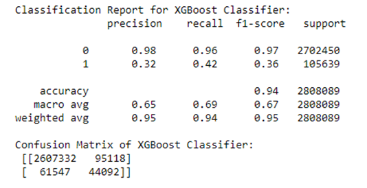
We trained an XGBoost (eXtreme Gradient Boosting) classifier on the dataset. Delinquency poses an imbalanced class problem because only about 2–8% of all loans are delinquent. This leaves 92–98% of the remaining loans remaining current on their payments and makes it tougher for classifiers to learn about the patterns reliably. Binary classification works best when the two classes are in balance. To overcome this, we oversampled the class with the fewest instances using a Python sklearn module known as RandomOverSampler.
The following code example from a Python notebook automates training an XGBoost classifier.First, merge the main mortgage loan acquisition data frame, df_acq, with the loan performance data frame which contains delinquency status, df_delinq4 (meaning the up to the 4th month without payment), using the Pandas-like RAPIDS-cuDF merge. Then, move the default column over to y and obtain the X_train, X_test, y_train, and y_test sub-data frames for training and testing. Having prepared and randomly split the training and test sections of the data, add in RandomOverSampler to help address the class imbalance problem and then prepare to call the routines to define, train, and evaluate the model. Of course, a best practice would entail a hyperparameter search. We did dedicate runs to that goal and found that the tuned classifier matched our hand-tuned one in accuracy. The notebook from a loan default article inspired our work with key modifications. The use of tree_method = ‘gpu_hist’ asks XGBoost to run on the GPU. RAPIDS includes a number of approaches to accelerate hyperparameter optimization. For more information, see Predicting Loan Defaults in the Fannie Mae Data Set and Use RAPIDS with Hyper Parameter Optimization.
df = merge(df_acq, df_delinq4, on='LoanID', how='outer')
...
y = df['default'].values
X = df.drop(['Default','LoanID'], axis=1).values
X_train, X_test, y_train, y_test = train_test_split(X, y, ...)
ros = RandomOverSampler(sampling_strategy=.90)
...
model = xgb.XGBClassifier(n_estimators = 500, max_depth = 4, n_jobs = 4, tree_method = 'gpu_hist')
model.train(...(X_train), ...(y_train))
probs = model.predict(xtest, pred_contribs=False)
An XGBoost classifier was developed as part of a Python Jupyter notebook to examine the predictability of loan delinquencies. We focus on XGBoost in this post. Given a dataset with stimulus variables and the default output variable, there is a limit to the predictability in the rows of data. Our results in Figure 2 are from a run of 11.2 million individual mortgages from 2007 to 2012 with a subset of 2.8 million loans residing in the test set. Using a customized threshold on the emitted probability of default helped to balance the precision and recall more evenly than using the standard value of 0.5.
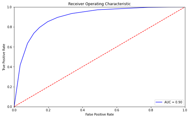
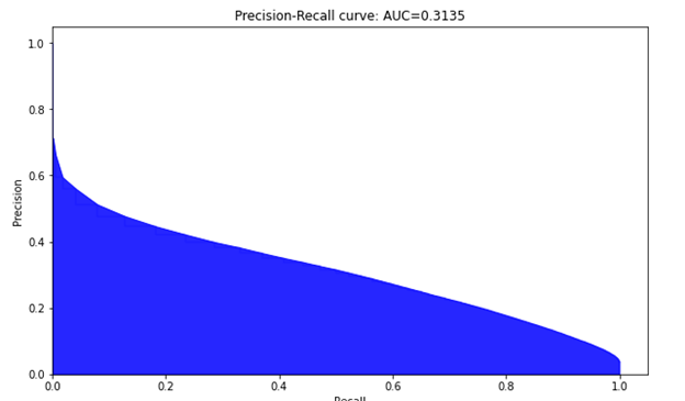
As mentioned earlier, you oversample the less frequent class to build a more balanced training set. Then, define the classifier, fit it, and obtain the predictions whose results are shown in Figure 3 and 4. This somewhat parallels work done on another mortgage dataset by the Bank of England, Machine Learning Explainability in Finance: An Application to Default Risk Analysis, also referred to as the 816 paper. In fact, even though a UK dataset was used in that paper and a US dataset for this post with slightly different features and machine learning classifiers, the ROC and Precision recall curves in their Figure 3 are similar to our Figures 3 and 4.
Explainability
Now that we have a model, and we’re confident that it generates decent predictions, we’d like to understand more about how and why it works. The current explanation techniques used in ML are Feature Importance and linear explanation techniques such as LIME (Local Interpretable Model-Agnostic Explanation) and Shapley values. For example, in predictions using a relatively simple multiple linear regression model, the set of \(\beta\)s provides all the explanation needed. As models get more complex, explainability becomes more complex too. For more information, see “Why Should I Trust You?”:Explaining the Predictions of Any Classifier and A Unified Approach to Interpreting Model Predictions.
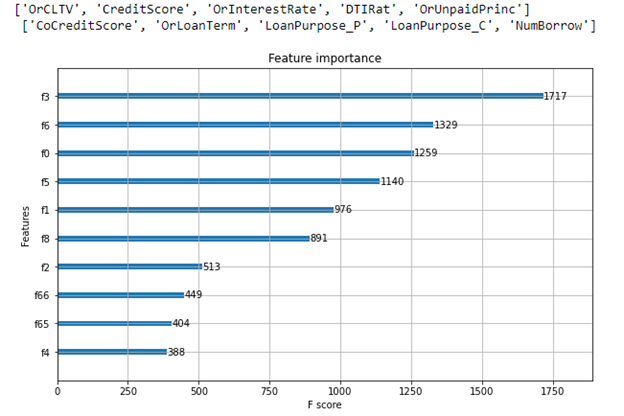
Traditionally, feature importance is reported to help explain the features used most to make decisions. A feature importance report is one of the benefits of using decision trees. With decision trees such as the XGBoost classifier, as the decision tree gets expanded via splits from the initial single node to hundreds of nodes, node impurity is not desired when a split occurs to gain accuracy.
Feature importance is the decrease in node impurity weighted by the chance of reaching that node. The most effective nodes are those that cause the best reduction in impurity and represent the largest number of samples in the data population. For more information, see Scikit Learn – Feature Importance Calculation in Decision Trees. For example, a solid decrease in the node impurity combined with a high probability of reaching the nodes splitting on that feature yields a high feature importance. This is what is behind a feature importance report like Figure 5. A feature’s importance report tells us which features in aggregate were influential to building the classifier but being an unsigned number, it does not intuitively tell us how the binary classification prediction is related to the value of the feature directionally.
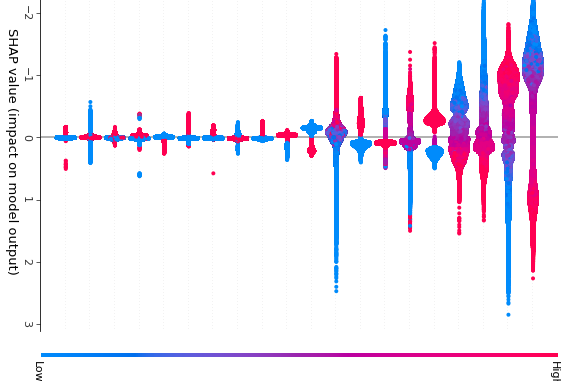
There appears to be consensus building in the data science community that Shapley values offer the most appealing explanations for the more advanced ML and DL predictions. For more information, see TreeExplainer, DeepExplainer, Gradient Explainer, KernelExplainer. There is also a strong mathematical basis for Shapley values which adds an element of rigor to their appeal. Shapley values highlight the marginal contributions of the various input factors on the resulting prediction, providing a simple explanation for any individual prediction. The calculations to find the Shapley values are computationally intense, but they are useful enough that they are becoming more widespread despite that. AI Software vendors such as Domino Data Labs, H20, and Fiddler.AI plus the wide availability of the SHAP() library, are promoting the use of Shapley value packages in Python. The explanations these provide give more transparency to help people understand predictions. For more information, see SHAP and LIME Python Libraries: Part 1 – Great Explainers, with Pros and Cons to Both.
In general, we’d like to be able to explain a single prediction and justify how the features led to that prediction. The feature explanations of SHAP sum up to the prediction for a single row, and we can aggregate across rows to explain a whole model. For regulatory purposes, this means that a model can provide a human-interpretable explanation for any output, favorable or adverse.
The benefits of having this explanation transparency is easy to see in the Bank of England paper. The authors call their approach Quantitative Input Influence (QII) and it is used for linear logistic and gradient boosted tree ML prediction models. The Shapley values are computed where the data set consists of 6 million loans in the U.K. with an approximate 2.5% default rate. The question arises: what factors contribute most to the defaults? Not only do the authors illustrate the intuitive power of the explanations, they also make observations which financial modelling practitioners should take note of regarding the ability to engineer adequate accuracy, precision, and recall for default prediction with their precision-recall curve results. Common loan attributes such as Loan-to-Value (LTV) ratio, income level, and interest rate come out near the top in the explanations for both models used. These familiar factors can be easily recognized by anyone who holds a mortgage or works in the debt instrument domain.
While speeding up classifiers using GPUs is well-covered in recent years, most recently with the same FNMA loan performance dataset, few studies have focused on GPU acceleration of Shapley values. The papers by Gerber and Denadai discuss the use of GPUs for training the classifier but not specifically for computing the Shapley values. For more information see Cake or Math: A Data/Science Blog and Interpretability of Deep Learning Models Towards Data Science. Depending upon the type of ML classifier, logistic, tree-based, or neural, there is a package available to compute Shapley values in a fashion tailored to the classifier. For example, for the XGBoost classifier the following code example retrieves and plot the Shapley values:
expl = shap.TreeExplainer(model)
shap_values = expl.shap_values(X_test_df)
shap.summary_plot(shap_values, X_test_df)
As Gerber explains in his paper, the basic equation for the set of Shapley values from game theory is a combinatorial approach, evaluating the contribution of each feature with and without it. This implies an \(O(2^n)\) algorithm complexity as subsets \(S\) such that \(S \subseteq F\backslash {i}\) (where \(F \backslash {i}\) is the feature set without feature \(i\)) so \(|F|\) Shapley values, each of which are computed with and without \(i\), the feature under study, contain a sum of \(2^ {|F|-1}\) terms. This formula is exponential in time-complexity, which can quickly become intractable for larger values of \(|F|\):
\(\varphi_i = \Sigma_{S \subseteq F \backslash { i }} { {|S|!(|F|-|S|-1)!}\over {|F|!}} (v(S \cup {i}) – v(S))\)
In this formula, \(v(S)\) is the payoff of player set \(S\). When computing \(\varphi_i\), the number terms is astronomical for ML with the possibly large number of features.
The good news is that for tree-based classifiers such as XGBoost, a special algorithm, TreeExplainer, reduces the complexity from \(O(T \ L \ 2^n)\) to \(O(T\ L\ D^2)\) where \(n\) is the number of features, \(T\) is the number of trees, \(L\) is the maximum number of leaves and \(D\) is the maximum tree depth. This converts the TreeExplainer process into a tractable process that can then be GPU-accelerated.
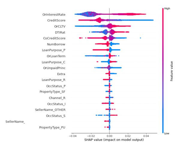
For the sake of illustration, say that there are only \(|F|\) = 4 features in our model to predict 0 or 1, whether the mortgage will default. The four features could be the numeric features OrInterestRate, CreditScore, OrCLTV, DTIRat, for example, which are the features with the most impact in Figure 6. In this case, we are interested in four Shapley values \(\varphi_i\) and they are additive for the final prediction.
Faster explainability
For this post, as it is public data, you have access to as many as 37 million loans with a set of FNMA mortgage loan key attributes and the associated monthly loan performance data. For more information, see Mortgage Data in the RAPIDS Demos. The loan performance detail records number over the half-a-billion range even when sampling the past decade of US loans. There is a 22x speedup on the GPU for computing Shapley values over the CPU. For more information, see GPUTreeShap: Fast Parallel Tree Interpretability.
Figure 7 shows the time required to read the input datasets, merge the two datasets, fit the model, predict the test values using the model, and generate the Shapley values on an NVIDIA DGX-1 machine with dual Xeon E5-2698 v4 CPU at 2.20GHz, a single V100 GPU on that DGX-1. The Python steps are being run in single-threaded mode.
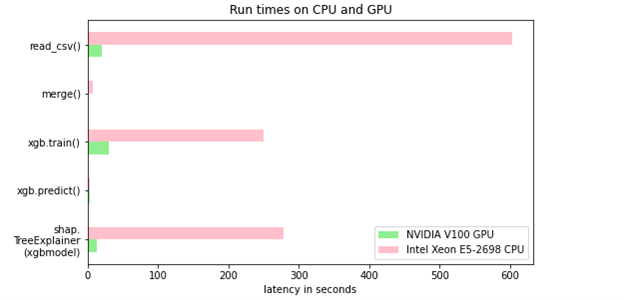
Table 1 quantifies the speedups shown earlier and underscores the benefit of GPU acceleration.
| CPU only | NVIDIA V100 GPU | Speedup Factor | |
| Read csv files | 603.0 sec. | 20.6 sec. | 29X |
| Perform merge() | 7.75 sec. | 0.1 sec. | 78X |
| Perform classifier fit() | 250.1 sec. | 30.0 sec. | 8X |
| Perform classifier predict() | 3.6 sec. | 3.6 sec. | 1X |
| Perform shap.TreeExplainer(model). shap_values(X_test_df) | 278.9 sec. | 12.5 sec. | 22X |
Next steps
In this post, we discussed how to use RAPIDS to GPU-accelerate the complete default analytics workflow: load and merge data, train a model to predict new results, and explain predictions of a financial credit risk problem using Shapley values. As AI matures, explaining the model predictions will become increasingly important, and being able to do it quickly and economically enables huge benefits.
- Visit the NVIDIA GPU Cloud (NGC) repository of containers to help build AI solutions.
- Attend the next NVIDIA GTC to share ideas and technology solutions.
- Comment on this post or in the forums.
