
This tutorial is the fourth installment of the series of articles on the RAPIDS ecosystem. The series explores and discusses various aspects of RAPIDS that allow its users solve ETL (Extract, Transform, Load) problems, build ML (Machine Learning) and DL (Deep Learning) models, explore expansive graphs, process signal and system log, or use SQL language via BlazingSQL to process data.
It’s been over 60 years [at the time of this writing] since the term Machine Learning (ML) was introduced. Since then, it has established a prominent place at the intersection between computer science, statistics, and econometrics. It is not that hard to imagine that nowadays virtually every human with a smartphone is using some form of machine learning every single day (if not every minute). Our preferences are modeled when we access the Internet so we are shown more relevant products, our opponents are more intelligent when we play a game, or a smartphone can recognize our face and unlock our phone.
Accelerate machine learning pipelines with RAPIDS cuML
Thus, when RAPIDS was introduced in late 2018, it arrived pre-baked with a slew of GPU-accelerated ML algorithms to solve some fundamental problems in today’s interconnected world. Since then, the palette of algorithms available in cuML (shortened from CUDA Machine Learning) has been expanded, and the performance of many of them has been taken to ludicrous levels. All while maintaining the familiar and logical API of scikit-learn!

In the previous posts we showcased other areas:
- In the first post, the python pandas tutorial, we introduced cuDF, the RAPIDS DataFrame framework for processing large amounts of data on an NVIDIA GPU.
- The second post compared similarities between cuDF DataFrame and pandas DataFrame.
- In the third post, data processing with Dask, we introduced a Python distributed framework that helps to run distributed workloads on GPUs.
In this tutorial, we will introduce and showcase the most common functionality of RAPIDS cuML.
Using cuML helps to train ML models faster and integrates perfectly with cuDF. Thanks to such tight integration, the end-to-end time to estimate a model is significantly reduced. This, in turn, allows interactively to engineer features and test new models and/or optimize their hyperparameters leading to better defined and more accurate models and enabling the ability to retrain the models more frequently.
To aid in getting familiar with using cuML, we provide a handy cuML cheatsheet that can be downloaded here.
Using GPUs to build statistical models
Estimating statistical models boils down to finding a minimum value of a loss function—or, inversely, a maximum value of the reward function—given a set of features (independent variables) and ground truth (or a dependent variable). Many algorithms exist that help finding roots of equations, some of them reaching back to the 17th century (see Newton-Rhapson algorithm) but all of them have one thing in common: ultimately all the features and the ground truth need to have a numerical representation.
Effectively, no matter whether we are building a classical ML model, try to estimate the latest-and-greatest Deep Learning model, or process an image, our computer will be dealing with a large matrix of numbers and apply some algorithms to it. GPUs, with thousands of cores, were made with that particular application in mind: to parallelize the processing of large matrices. For example, the frames when we play a game are rendered so fast you cannot perceive any lag on the screen, a filter we apply to an image does not take one day to finish, or, as we might have guessed, the process of estimating a model is significantly sped up.
GPUs made the first forays into the world of Machine Learning by speeding up the estimation of Deep Learning models since the amount of data and the size of these models require an outrageous amount of computation. DL models, however, while capable of solving some sophisticated modeling problems, are quite often overkill for other simpler problems with well-established solutions.
Thus, if our dataset is large, and we want to go from reading our data to having an estimated regression or classification model in minutes rather hours or days, RAPIDS is the right tool
Regression and classification – the backbone of machine learning
Regression and classification problems are intimately related, differing mostly in the way how the loss function is derived. In the regression model, we normally want to minimize the distance (or squared distance) between the value predicted by the model and the target, while the aim of a classification model is to minimize the number of misclassified observations. To further the argument that either regression or classification are based on virtually the same underlying mathematical model, we have a family of models, live Support-Vector Machines or ensemble models (like Random Forest or XGBoost) that can be applied to solve either.
The cuML package has a whole portfolio of models to solve regression or classification problems. And all but a few implement exactly the same API call that simplifies testing different approaches. Consider estimating a linear regression, and then trying out a ridge or lasso: all we have to do is to change the object we create.
You can estimate a Linear Regression model in two lines of code:
model = cuml.LinearRegression(fit_intercept=True, normalize=True)
model.fit(X_train, y_train).predict(X_test)
Estimating a Lasso Regression (as a reminder, it provides an L1 regularization on the coefficients) requires changing the object:
model = cuml.Lasso(fit_intercept=False, normalize=True)
model.fit(X_train, y_train).predict(X_test)
A similar pattern can be found when trying to estimate a classification model: a logistic regression can be estimated as follows:
model = cuml.LogisticRegression(fit_intercept=True)
model.fit(X_train, y_train).predict(X_test)
Unlike regression models, some of the estimated classification models can also output probabilities of belonging to a certain class.
model.predict_proba(X_test)
Check the cuML-cheatsheet to further explore the regression and classification models of RAPIDS, or use cuML-notebooks to try it.
Finding pattern in data
Many times, the target variable or a label is not readily available in a dataset produced in a real-world scenario. Labeling datasets for machine learning has even become a business model on its own. However, clustering data is an example of statistical modeling without a teacher or unsupervised modeling that does not require having the ground truth but rather finds patterns in data.
One of the simplest yet powerful segmentation models is k-means. k-means, given the observations and their features, finds clusters that maximize the cluster homogeneity (how similar the observations are within the same cluster) while at the same time maximizing the heterogeneity (dissimilarity) between clusters. While the k-means algorithm is quite efficient and scales well to a relatively large dataset, estimating a k-means model using RAPIDS we gain further performance improvements.
k_means = cuml.KMeans(n_clusters=4, n_init=3)
k_means.fit_transform(X_train)
One of the drawbacks of k-means is that it requires explicitly stating the number of clusters we expect to see in the data. DBSCAN, also available in cuML, does not have such requirements.
dbscan = cuml.DBSCAN(eps=0.5, min_samples=10)
dbscan.fit_predict(X_train)
DBSCAN is a density-based clustering model. Unlike k-means, DBSCAN can leave some of the points unclustered, effectively finding some outliers that do not really match any of the patterns found.
Dealing with high-dimensional data
For many real-life phenomena, we have no ability to collect enough data to estimate a statistically significant machine learning model, or the nature of the phenomenon makes the data extremely high-dimensional and sparse. For example, some rare diseases can have many features describing the patient compared to the number of observed patients we can collect the data from, putting us effectively in a statistical impasse. On the other hand, we might have billions of records but the feature space can be hundreds of millions big, making estimating the model impractical at best.
Dimensionality reduction is one of the techniques to reduce the number of features and keep only those that are highly correlated with the target, or can explain most of the target’s variance. PCA, or Principal Component Analysis, is one of the oldest techniques that projects a high-dimensional feature space onto an orthogonal hyperplane where each feature is guaranteed to be independent of each other, and then retains only some number of them that explain most of the variance of the target. cuML has a fast implementation of PCA that we can estimate in one line of code.
pca = cuml.PCA(n_components=2)
The above code takes a dataset and retrieves only the first two principal components that can be easily plotted. An example below retrieved 2 principal components from a dataset created using cuML.
X, y = cuml.make_blobs(
    n_samples=1000
    , centers=4
    , n_features=50
    , cluster_std=[1.0, 5.0, 10.0, 0.5]
    , random_state=np.random.randint(1e9)
)
We have 50 features, 1000 observations, and four clusters. Running PCA to retrieve the top two principal components and plotting the results shows the following image.
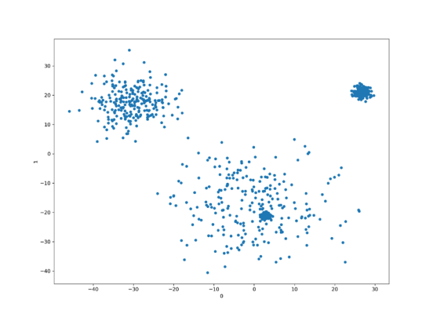
So, instead of 50 features, we can use only two and most likely still build a decent model. Of course, not many models would be able to find four clusters here, but the separation between 3 of them is quite profound.
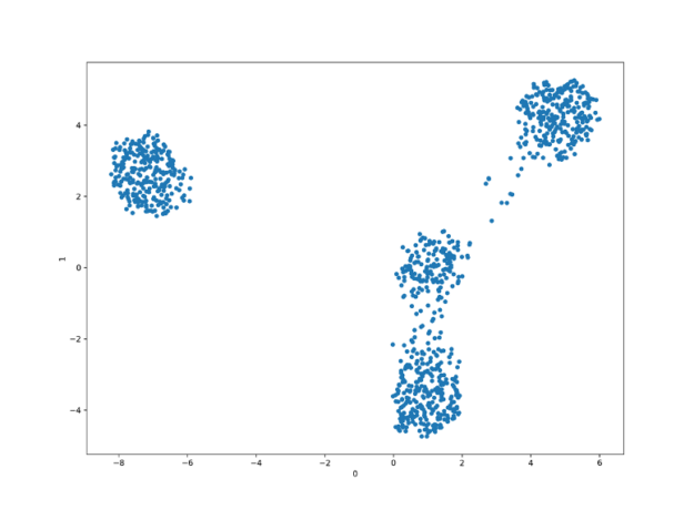
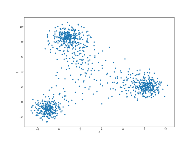
umap = cuml.UMAP(n_neighbors=10, n_components=2)
tsne = cuml.TSNE(n_components=2, perplexity=500, learning_rate=200)
Both UMAP and t-SNE produce better-separated clusters than the PCA, with the UMAP being the ultimate winner being able to almost ideally retrieve linearly separable four clusters of points.
t-SNE produces linearly separable clusters but seems to be missing one of them, just like PCA.
Download the cuML cheatsheet to help create your own GPU-accelerated ML pipelines!
