Perception Model Training for Autonomous Vehicles with Tensor Parallelism

Due to the adoption of multicamera inputs and deep convolutional backbone networks, the GPU memory footprint for training autonomous driving perception models is large. Existing methods for reducing memory usage often result in additional computational overheads or imbalanced workloads.

This post describes joint research between NVIDIA and NIO, a developer of smart electric vehicles. Specifically, we explore how tensor parallel convolutional neural network (CNN) training can help reduce the GPU memory footprint. We also demonstrate how NIO has improved the training efficiency and GPU utilization of perception models for autonomous vehicles.

Perception model training for autonomous vehicles

Autonomous driving perception tasks extract features by using multicamera data as input and CNNs as the backbone. The forward activations of CNNs are feature maps of shape (N, C, H, W), where N, C, H, W are number of images, number of channels, height, and width, respectively. The activations need to be saved for backward propagation, thus the training of the backbone usually consumes significant memory. 

For example, assuming six camera RGB inputs with 720 pixel resolution and the batch size set to 1, the input shape of the backbone network is (6, 3, 720, 1280). For backbone networks such as RegNet or ConvNeXt, the memory footprint of the activations is much larger than the memory usage of model weights and optimizer states, and may exceed the limit of GPU memory size. 

According to research by the NIO Autonomous Driving Team, adopting deeper models and higher image resolution can significantly improve perception accuracy, especially for recognizing small and distant targets. Powered by 11 eight-megapixel HD cameras, the NIO Aquila Super Sensing system generates 8 GB of image data per second. 

Demands on GPU memory optimization

The deep model and high-resolution input put higher demands on GPU memory optimization. Current techniques for addressing the excessive GPU memory footprint of activations include gradient checkpointing, which retains the activations of only some of the layers during forward propagation. For other layers, the activations are recalculated during backpropagation. 

Despite saving GPU memory, it increases computing overhead and slows down the model training. In addition, setting gradient checkpoints usually requires the developer to select and debug based on the model structure, bringing additional costs to the model training.

NIO has also used pipelined parallelism, where the neural network was segmented equally based on GPU memory overhead and deployed to multiple GPUs for training. This approach distributes the storage requirements equally across multiple GPUs. However, it causes significant load imbalance between GPUs and insufficient utilization of some GPUs.

Tensor parallel CNN training based on PyTorch DTensor

Considering these factors, NVIDIA and NIO have jointly designed and implemented tensor parallel CNN training that slices the inputs and intermediate activations across multiple GPUs. The model weights and optimizer states are replicated on each GPU just like the practice of data parallel training. This approach reduces GPU memory footprint and bandwidth pressure for individual GPUs. 

Introduced in PyTorch 2.0, DTensor provides primitives to express tensor distribution, such as sharding and replication. It enables users to easily perform distributed computing without explicitly calling communication operators, as the underlying implementation of DTensor has already encapsulated communication libraries such as NVIDIA Collective Communications Library (NCCL). 

With the abstraction of DTensor, users can easily build various parallel training strategies, including tensor parallel, distributed data parallel, and fully sharded data parallel. 

Implementation

Taking the CNN model for vision tasks, ConvNeXt-XL as an example, we’ll demonstrate the tensor parallel CNN training. Place DTensor as follows:

• Model parameters: Replicate
  • Repetitively placing on each GPU. The model contains 350 million parameters and consumes 1.4 GB of GPU memory when stored in FP32.
• Model inputs: Shard(3) 
  • Slicing the W dimension of (N, C, H, W). Place the input slices on each GPU. For example, Shard(3) for input of shape (7, 3, 512, 2048) on four GPUs generates four slices of shape (7, 3, 512, 512).
• Activations: Shard(3) 
  • Slicing the W dimension of (N, C, H, W). Place the activation slices on each GPU.
• Gradients of model parameters: Replicate 
  • Repetitively placing on each GPU.
• Optimizer states: Replicate 
  • Repetitively placing on each GPU.

The preceding configurations can be done through the APIs provided by DTensor. The user simply specifies the placement of model parameters and model inputs, and the placement of other tensors will be generated automatically. 

To enable tensor parallel training, propagation rules should be registered for the convolution operators aten.convolution and aten.convolution_backward. This will determine the placement of the output DTensor based on the placement of the input DTensor:

• aten.convolution
  • Input placement is Shard(3), weight and bias placement is Replicate, output placement is Shard(3)
• aten.convolution_backward
  • grad_output placement is Shard(3), weight and bias placement is Replicate, grad_input placement is Shard(3), grad_weight and grad_bias placements are _Partial

DTensor with _Partial placement automatically performs a reduction operation when its value is used and the default reduction operator is sum.

Next is the forward and backward implementation of the tensor parallel convolution operator. Because the activations are sliced across multiple GPUs, local convolution on one GPU may need edge data of activations from neighboring GPUs, which requires inter-GPU communication. In the ConvNeXt-XL model, this problem is not seen in the convolution in its downsampling layer, while it must be handled in the depthwise convolution in Block. 

If no data exchange is required, users can call the forward and backward operators of the convolution directly and pass in the local tensors. If exchange of the tensor edge data of local activations is required, use the convolution forward and backward algorithms shown in Figures 1 and 2. We omit N and C dimensions in the figures, and assume that the convolution kernel size is 5×5, padding is 2, and stride is 1. 

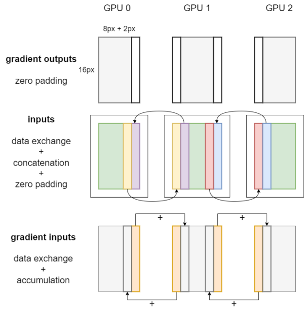
As shown in Figure 1, when the convolution kernel size is 5×5, padding is 2, and stride is 1, the local input on each GPU should take the input edge of width 2 from its neighboring GPUs and concatenate the received edge data to itself. In other words, inter-GPU data exchange is needed to ensure the correctness of tensor parallel convolution. This data exchange can be enabled by calling the NCCL send-receive communication operator encapsulated in PyTorch. 

It’s worth mentioning that some of the padding of the convolution operator isn’t needed when the activations are sliced on multiple GPUs. The invalid pixels introduced by the unwanted paddings in the outputs should be cropped after the local convolution forward propagation is completed, as shown by the blue-patterned bars in Figure 1.

Figure 2 shows the workflow of backpropagation for tensor parallel convolution. First, zero padding is applied on the gradient outputs, which corresponds to the cropping operation on the outputs during forward propagation. As for ‌local inputs, the same procedures of data exchange, concatenation, and padding are conducted. 

After that, weight gradients, bias gradients, and gradient inputs can be obtained by calling the convolution backward operator on each GPU.

The placement of weight gradients and bias gradients is _Partial, so their values will be automatically reduced across multiple GPUs when they are used. The placement of gradient inputs is Shard(3). 

Finally, the edge pixels of local gradient inputs are sent to neighboring GPUs and accumulated at the corresponding positions, as shown by the orange bars in Figure 2.

In addition to the convolutional layer, ConvNeXt-XL has several layers that need to be handled to support tensor parallel training. For example, propagation rules should be registered for the aten.bernoulli operator used by the DropPath layer. This operator should be placed in the distributed region of the random number generation tracker to ensure consistency across GPUs. 

All the code has been merged into the main branch of the PyTorch GitHub repo, so users can implement tensor parallel CNN training by directly calling the high-level APIs of DTensor.

Benchmark results of training ConvNeXt with tensor parallelism

We conducted the benchmark on the NVIDIA DGX AI platform to explore the speed and GPU memory footprint of ConvNeXt-XL training. The techniques of gradient checkpointing and DTensor are compatible, and GPU memory usage can be reduced more significantly by combining the two techniques. 

The baseline of this benchmark is using the PyTorch native tensor on one NVIDIA GPU with input size (7, 3, 512, 1024). Without gradient checkpointing, the GPU memory footprint is 43.28 GiB and a single training iteration takes 723 ms. With gradient checkpointing, these are 11.89 GiB and 934 ms, respectively. 

The complete results are shown in Figures 3 and 4. The global input shape is (7, 3, 512, W), where W varies from 1024 to 8192. The solid lines are results without gradient checkpointing, while the dashed lines are results with gradient checkpointing. 

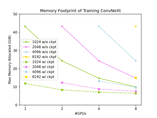
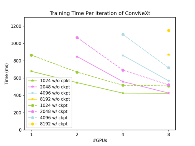
As shown in Figure 3, slicing the activations using DTensor can effectively reduce the GPU memory footprint of ConvNeXt-XL training, and it can be reduced to a very low level when we apply both DTensor and gradient checkpointing. As shown in Figure 4, the tensor parallel approach has good weak scalability and offers good strong scalability when the problem size is large enough. This looks into the case where gradient checkpointing is not used:

• A single iteration takes 937 ms in the case of global input of shape (7, 3, 512, 2048) on two GPUs.
• A single iteration takes 952 ms in the case of global input of shape (7, 3, 512, 4096) on four GPUs.
• A single iteration takes 647 ms in the case of global input of shape (7, 3, 512, 4096) on eight GPUs.

Conclusion

Using DTensor to implement tensor parallel CNN training provides a solution to effectively improve training efficiency on NADP (NIO Autonomous Driving Development Platform), an R&D platform dedicated to the core autonomous driving service of NIO. NADP delivers high-performance computing and full-chain tools to process hundreds of thousands of daily inference and training tasks, ensuring the ongoing evolution of active safety and driver assistance functions. 

This key approach enables NADP to perform parallel computing at a 10,000-GPU scale. It improves GPU utilization, reduces the cost of model training, and enables a more flexible model structure. Benchmarks show that this approach performs well in NIO’s autonomous driving scenarios and effectively addresses the challenges of training large vision models.

Tensor parallelism training for CNNs based on PyTorch DTensor can significantly reduce the memory footprint and maintain good scalability. We anticipate that this approach will make perception model training more widely accessible by fully leveraging the computing power and interconnects of multiple GPUs.

For more details, visit the PyTorch GitHub repo.