Autonomous driving demands safety, and a high-performance computing solution to process sensor data with extreme accuracy. Researchers and developers creating deep neural networks (DNNs) for self driving must optimize their networks to ensure low-latency inference and energy efficiency. Thanks to a new Python API in NVIDIA TensorRT, this process just became easier.
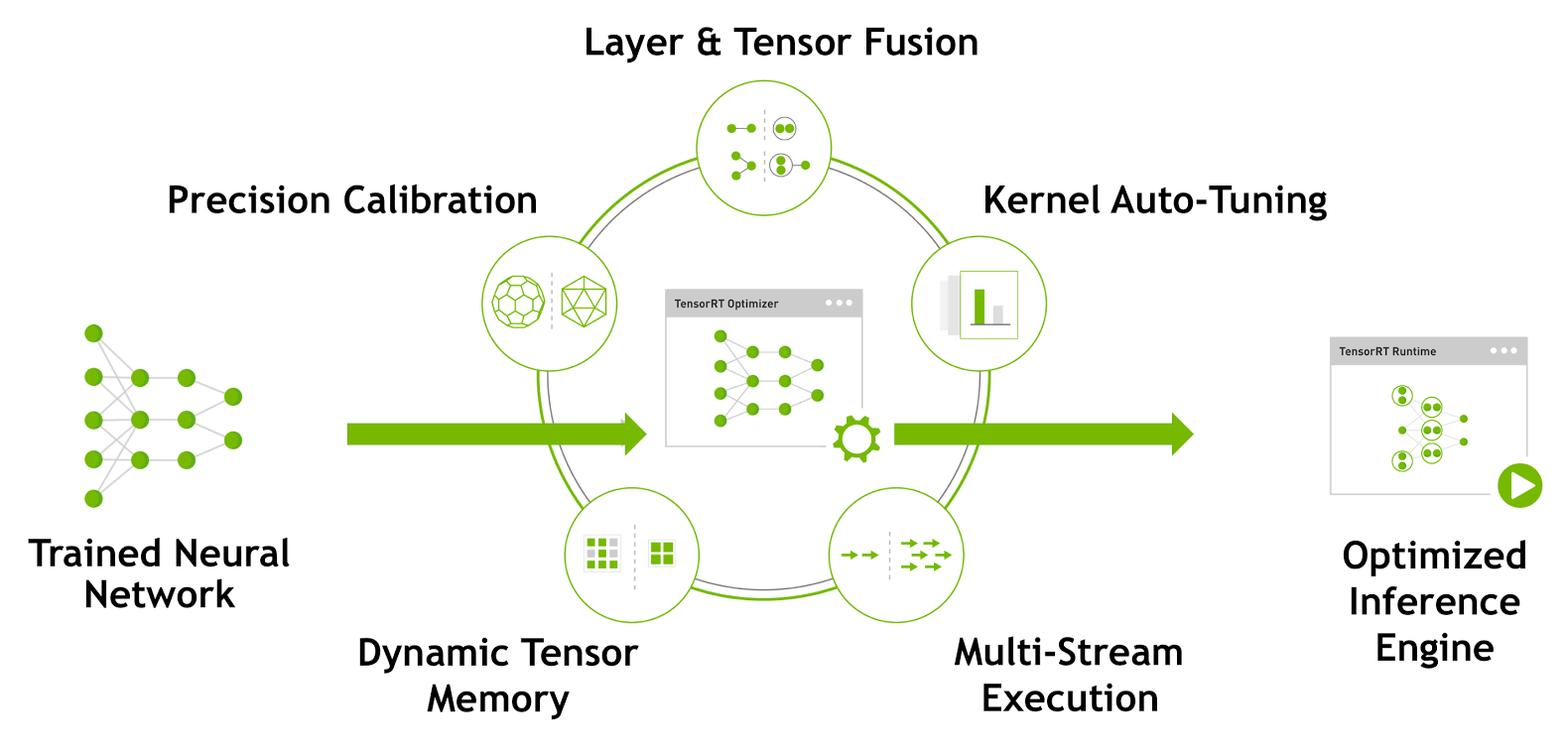
TensorRT is a high-performance deep learning inference optimizer and runtime engine for production deployment of deep learning applications. Developers can optimize models trained in TensorFlow or Caffe to generate memory-efficient runtime engines that maximize inference throughput, making deep learning practical for latency-critical products and services like autonomous driving..
The latest TensorRT 3 release introduces a fully-featured Python API, which enables researchers and developers to optimize and serialize their DNN using familiar Python code. With TensorRT 3 you can deploy models either in Python, for cloud services, or in C++ for real-time applications such as autonomous driving software running on the NVIDIA DRIVE PX AI car computer.
In this post, I will show you how to use the TensorRT 3 Python API on the host to cache calibration results for a semantic segmentation network for deployment using INT8 precision. The calibration cache then can be used to optimize and deploy the network using the C++ API on the DRIVE PX platform.
The Cityscapes Dataset and Fully Convolutional Network

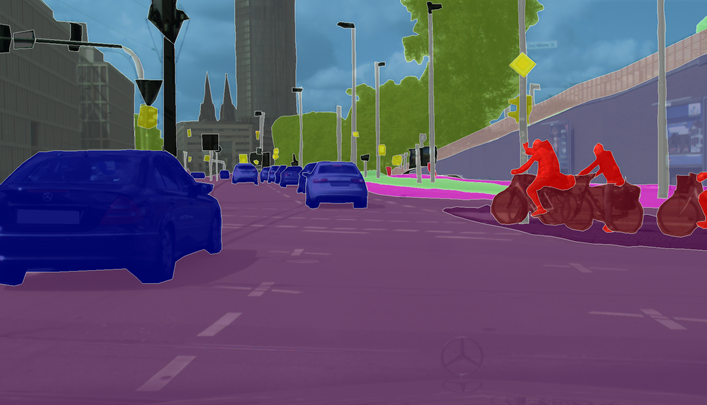
The Cityscapes Dataset [Cordts et al. 2016] is designed for semantic segmentation of urban autonomous driving scenarios. Figure 2 shows sample images from the dataset. The dataset has a total of 30 different classes, grouped into 8 different categories. For the purpose of evaluating performance, I use 19 classes and 7 categories, as Figure 3 shows.
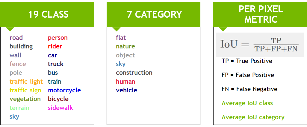
For evaluation, I use the IoU (Intersection-over-Union) metric, which provides two average scores, one for the class and the other for the category.

To demonstrate the capabilities of TensorRT, I designed a variant of the fully convolutional network (FCN [Long et al. 2015]) based on VGG16, as Figure 4 shows. The network consists of a VGG16-based encoder and two upsampling layers implemented using a deconvolutional layer. I trained the network on the Cityscapes Dataset using NVIDIA DIGITS with a Caffe [Jia et al. 2014] backend.

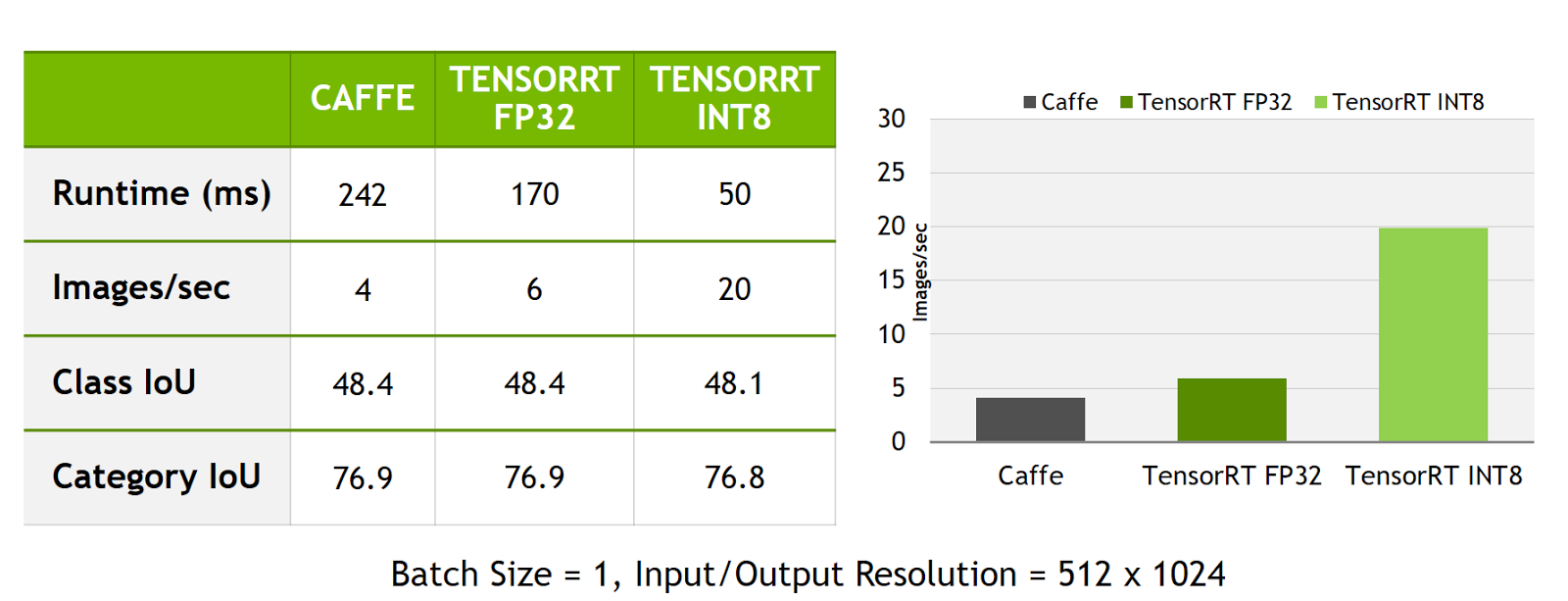
This network is designed to take a 512×1024 input image and produce a per-pixel classification result, as Figure 5 shows. The trained network achieves an average IoU class score of 48.4 and an average IoU category score of 76.9. If I directly use Caffe with cuDNN to run inference on one of the DRIVE PX AutoChauffeur GPUs (Pascal), this network achieves approximately 242 ms latency and about 4 images/sec throughput. At a speed of 35 mph, 242 ms equates to about 12 feet of driving distance. This level of performance is not good enough for making timely decisions for autonomous driving. Let’s take a look at how we can do better.
As a first step, optimizing the network using TensorRT using FP32 precision provides a good speedup. Just by using TensorRT, I achieved 170 ms latency and about 6 images/sec throughput. This is an impressive 50% improvement over Caffe, but TensorRT can optimize the network further.
The following sections demonstrate how to use TensorRT to improve the inference performance of this network using INT8 reduced precision, while maintaining the good accuracy of the original FP32 network.
INT8 Inference and Calibration
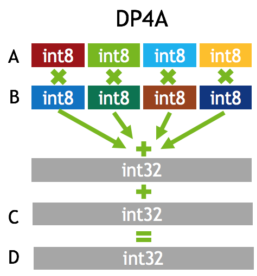
The Pascal dGPU in DRIVE PX AutoChauffeur is capable of executing 8-bit integer 4-element vector dot product (DP4A, see Figure 6) instructions to accelerate deep neural network inference. While this new instruction provides faster computation, there is a significant challenge in representing weights and activations of deep neural networks in this reduced INT8 format. As Table 1 shows, the dynamic range and granularity of representable values for INT8 is significantly limited compared to FP32 or FP16.
| Dynamic Range | Mininum Positive Value | |
|---|---|---|
| FP32 | -3.4×1038 ~ +3.4×1038 | 1.4 × 10−45 |
| FP16 | -65504 ~ +65504 | 5.96 x 10⁻⁸ |
| INT8 | -128 ~ +127 | 1 |
TensorRT provides a quick and easy way to take a model trained in FP32 and automatically convert the network for deployment with INT8 reduced precision with minimal accuracy loss. In order to achieve this goal, TensorRT uses a calibration process that minimizes the information loss when approximating the FP32 network with a limited 8-bit integer representation. For more information on how this algorithm works, please see the 8-bit Inference with TensorRT GPU Technology Conference presentation.
When preparing the calibration dataset, you should capture the expected distribution of data in typical inference scenarios. You want to make sure that the calibration dataset covers all the expected scenarios; for example, clear weather, rainy day, night scenes, etc. If you are creating your own dataset, we recommend creating a separate calibration dataset. The calibration dataset shouldn’t overlap with the training, validation or test datasets, in order to avoid a situation where the calibrated model only works well on the these datasets.
Let’s take a look at how you can use the new TensorRT Python API to create a calibration cache.
Creating a Calibration Cache Using the Python API
With the introduction of the TensorRT Python API, it is now possible to implement the INT8 calibrator class purely in Python. This example shows how to process image data and feed the calibrator. It should be simple to modify this example to support different types of data and networks in Python.
import pycuda.driver as cuda
import pycuda.autoinit
import numpy as np
from PIL import Image
import ctypes
import tensorrt as trt

CHANNEL = 3
HEIGHT = 512
WIDTH = 1024

class PythonEntropyCalibrator(trt.infer.EntropyCalibrator):
  def __init__(self, input_layers, stream):
    trt.infer.EntropyCalibrator.__init__(self)
    self.input_layers = input_layers
    self.stream = stream
  self.d_input = cuda.mem_alloc(self.stream.calibration_data.nbytes)
    stream.reset()

  def get_batch_size(self):
    return self.stream.batch_size

  def get_batch(self, bindings, names):
    batch = self.stream.next_batch()
    if not batch.size:
      return None

    cuda.memcpy_htod(self.d_input, batch)
    for i in self.input_layers[0]:
      assert names[0] != i

    bindings[0] = int(self.d_input)
    return bindings

  def read_calibration_cache(self, length):
    return None

  def write_calibration_cache(self, ptr, size):
    cache = ctypes.c_char_p(int(ptr))
    with open('calibration_cache.bin', 'wb') as f:
      f.write(cache.value)
    return None
The PythonEntropyCalibrator class is a Python implementation of an INT8 calibrator. This class is responsible for allocating CUDA memory and creating bindings for all input layers. It uploads the calibration input data to pre-allocated CUDA memory whenever get_batch() is called. The calibration batch size defines how many calibration images get processed at the same time for collecting the input distribution required to compute the correct scaling factor. The calibration batch size can be different from the max batch size parameter for inference. Using larger calibration batch size usually speeds up the calibration process and I recommend using the maximum batch size that can fit in GPU memory.
class ImageBatchStream():
  def __init__(self, batch_size, calibration_files, preprocessor):
    self.batch_size = batch_size
    self.max_batches = (len(calibration_files) // batch_size) + \
                       (1 if (len(calibration_files) % batch_size) \
                        else 0)
    self.files = calibration_files
    self.calibration_data = np.zeros((batch_size, CHANNEL, HEIGHT, WIDTH), \
                                     dtype=np.float32)
    self.batch = 0
    self.preprocessor = preprocessor

  @staticmethod
  def read_image_chw(path):
    img = Image.open(path).resize((WIDTH,HEIGHT), Image.NEAREST)
    im = np.array(img, dtype=np.float32, order='C')
    im = im[:,:,::-1]
    im = im.transpose((2,0,1))
    return im

  def reset(self):
    self.batch = 0

  def next_batch(self):
    if self.batch < self.max_batches:
      imgs = []
      files_for_batch = self.files[self.batch_size * self.batch : \
                        self.batch_size * (self.batch + 1)]
      for f in files_for_batch:
        print("[ImageBatchStream] Processing ", f)
        img = ImageBatchStream.read_image_chw(f)
        img = self.preprocessor(img)
        imgs.append(img)
      for i in range(len(imgs)):
        self.calibration_data[i] = imgs[i]
      self.batch += 1
      return np.ascontiguousarray(self.calibration_data, dtype=np.float32)
    else:
      return np.array([])
ImageBatchStream is a helper class that takes care of file I/O, scaling of the image size, creating batch data for processing, reordering of the data layout as CHW format, and applying preprocessor functions, such as subtracting the image mean value.
The result of calibration can be saved to a cache file, so the optimized TensorRT runtime engine can be created without repeating the calibration process on the target. In this example, the generated file name is calibration_cache.bin, as handled in the write_calibration_cache function.
Once the calibrator class is prepared, the rest of the process can be streamlined with TensorRT’s new tensorrt.lite Python module, which is designed to abstract away many low-level details to make it easier for data scientists to use TensorRT. This package allows you to add pre- and post-processing functions, and makes it possible to leverage existing Python data pre-processing routines. In the following code, the function sub_mean_chw handles mean value subtraction as a pre-processing step and the function color_map handles mapping the output class ID to color for visualizing the output.
import glob
from random import shuffle
import numpy as np
from PIL import Image

import tensorrt as trt

import labels        #from cityscapes evaluation script
import calibrator    #calibrator.py

MEAN = (71.60167789, 82.09696889, 72.30508881)
MODEL_DIR = '/data/fcn8s/'
CITYSCAPES_DIR = '/data/Cityscapes/'
TEST_IMAGE = CITYSCAPES_DIR + 'leftImg8bit/val/lindau/lindau_000042_000019_leftImg8bit.png'
CALIBRATION_DATASET_LOC = CITYSCAPES_DIR + 'leftImg8bit/train/*/*.png'

CLASSES = 19
CHANNEL = 3
HEIGHT = 512
WIDTH = 1024

def sub_mean_chw(data):
  data = data.transpose((1,2,0)) # CHW -> HWC
  data -= np.array(MEAN) # Broadcast subtract
  data = data.transpose((2,0,1)) # HWC -> CHW
  return data

def color_map(output):
  output = output.reshape(CLASSES, HEIGHT, WIDTH)
  out_col = np.zeros(shape=(HEIGHT, WIDTH), dtype=(np.uint8, 3))
  for x in range (WIDTH):
    for y in range (HEIGHT):
    out_col[y,x] = labels.id2label[labels.trainId2label[np.argmax(output[:,y,x])].id].color
  return out_col
Here is the main function that puts all the codes together. The tensorrt.lite module provides high-level functions to convert Caffe and TensorFlow models to optimized engines using one function called tensorrt.lite.Engine.
def create_calibration_dataset():
  # Create list of calibration images (filename)
  # This sample code picks 100 images at random from training set
  calibration_files = glob.glob(CALIBRATION_DATASET_LOC)
  shuffle(calibration_files)
  return calibration_files[:100]

def main():
  calibration_files = create_calibration_dataset()

  # Process 5 images at a time for calibration
  # This batch size can be different from MaxBatchSize (1 in this example)
  batchstream = calibrator.ImageBatchStream(5, calibration_files, sub_mean_chw)
  int8_calibrator = calibrator.PythonEntropyCalibrator(["data"], batchstream)

  # Easy to use TensorRT lite package
  engine = trt.lite.Engine(framework="c1",
                           deployfile=MODEL_DIR + "fcn8s.prototxt",
                           modelfile=MODEL_DIR + "fcn8s.caffemodel",
                           max_batch_size=1,
                           max_workspace_size=(256 << 20),
                           input_nodes={"data":(CHANNEL,HEIGHT,WIDTH)},
                           output_nodes=["score"],
                           preprocessors={"data":sub_mean_chw},
                           postprocessors={"score":color_map},
                           data_type=trt.infer.DataType.INT8,
                           calibrator=int8_calibrator,
                           logger_severity=trt.infer.LogSeverity.INFO)

  test_data = calibrator.ImageBatchStream.read_image_chw(TEST_IMAGE)
  out = engine.infer(test_data)[0]
  test_img = Image.fromarray(out, 'RGB')
  test_img.show()
Within the Cityscapes dataset, there are separate training, validation and test sets, following the common practice for deep learning. However, this means that there is no separate calibration dataset put aside. Therefore you can randomly select 100 images from the training dataset to use as the calibration dataset, in order to illustrate how well the calibration process works. As you will see, the calibration algorithm can achieve good accuracy with just 100 random images!
Using a system containing an NVIDIA GPU with Compute Capability 6.1 (such as a Quadro P4000, Tesla P4 or P40), you can run the INT8 optimized engine to validate its accuracy. I recommend running the entire validation dataset to make sure that the small accuracy loss introduced by using reduced precision is acceptable. By running the Cityscapes evaluation script using all 500 validation images, I found that the calibrated INT8 model achieves 48.1 average class IoU and 76.8 average category IoU, compared to 48.4 and 76.9 in the original FP32 precision model.
Optimizing the INT8 Model on DRIVE PX
TensorRT builder implements a profiling-based optimization called kernel autotuning. This process requires the network to be optimized on the target device. We can use the calibration cache file generated from the host in this on-target optimization phase to generate an INT8 model without requiring the calibration dataset. You need to write a calibrator class that implements the readCalibrationCache function to tell the TensorRT to use the cached result as the following code shows.
class Int8CacheCalibrator : public IInt8EntropyCalibrator {
public:
  Int8CacheCalibrator(std::string cacheFile)
    : mCacheFile(cacheFile) {}
  virtual ~Int8CacheCalibrator() {}

  int getBatchSize() const override {return 1;}

  bool getBatch(void* bindings[], const char* names[], int nbBindings) override {
    return false;
  }

  const void* readCalibrationCache(size_t& length) override
  {
    mCalibrationCache.clear();
    std::ifstream input(mCacheFile, std::ios::binary);
    input >> std::noskipws;
    if (input.good()) {
      std::copy(std::istream_iterator(input),
      std::istream_iterator<char>(),
      std::back_inserter<char>(mCalibrationCache));
    }
    length = mCalibrationCache.size();
    return length ? &mCalibrationCache[0] : nullptr;
  }

private:
  std::string mCacheFile;
  std::vector<char> mCalibrationCache;
};
By taking advantage of INT8 inference with TensorRT, the model can now run in 50 ms latency or 20 images/sec on a single Pascal GPU of DRIVE PX AutoChauffeur. Figure 7 summarizes the performance obtained with TensorRT using FP32 and INT8 inference.
You can serialize the optimized engine to a file for deployment, and then you are ready to deploy the INT8 optimized network on DRIVE PX!
Get Your Hands on TensorRT 3
NVIDIA TensorRT is a high-performance deep learning inference accelerator that delivers low latency, high-throughput inference for deep neural networks. TensorRT 3 is available now for x86 systems. TensorRT 3 will be available for DRIVE PX 2 by mid-January 2018. If you would like to get it sooner, please contact your NVIDIA solution architect or representative. For additional details on using TensorRT on NVIDIA DRIVE PX, register for our webinar.
References
[Jia et al. 2014] Caffe: Convolutional Architecture for Fast Feature Embedding. Jia, Yangqing and Shelhamer, Evan and Donahue, Jeff and Karayev, Sergey and Long, Jonathan and Girshick, Ross and Guadarrama, Sergio and Darrell, Trevor (arXiv:1408.5093)
[Long et al. 2015] Fully Convolutional Networks for Semantic Segmentation. Jonathan Long, Evan Shelhamer, Trevor Darrell (CVPR 2015)
[Cordts et al. 2016] The Cityscapes Dataset for Semantic Urban Scene Understanding. Marius Cordts, Mohamed Omran, Sebastian Ramos, Timo Rehfeld, Markus Enzweiler, Rodrigo Benenson, Uwe Franke, Stefan Roth, Bernt Schiele (CVPR 2016)
