Optimizing Fraud Detection in Financial Services with Graph Neural Networks and NVIDIA GPUs

Fraud is a major problem for many financial services firms, costing billions of dollars each year, according to a recent Federal Trade Commission report. Financial fraud, fake reviews, bot assaults, account takeovers, and spam are all examples of online fraud and harmful activity.

Although these firms employ techniques to combat online fraud, the methods can have severe limitations. Simple rule-based techniques and feature-based algorithm techniques (logistic regression, Bayesian belief networks, CART, and others) aren’t adaptable enough to detect the full range of fraudulent or suspicious online behaviors. 

Fraudsters, for example, might set up many coordinated accounts to avoid triggering limitations on individual accounts. In addition, detecting fraudulent behavior patterns at scale is difficult due to the huge volume of data to sift through (billions of rows, tens of terabytes), the complexity of continually improving methodologies, and the scarcity of real cases of fraudulent activity required for training classification algorithms. For more details, see Intelligent Financial Fraud Detection Practices: An Investigation.

Although the cost of fraud is billions of dollars per year, there are very few fraudulent transactions among many legitimate transactions, leading to an imbalance in labeled data, when it is even available.  Detecting fraud becomes even more complex in the financial services industry, due to security concerns around personal data and the need for transparency in the methods used to detect the fraudulent activity. 

An explainable model enables fraud analysts to understand what inputs the algorithm used in the analysis and the reason(s) for flagging the transaction, building a stronger trust in the system. Additional benefits include the ability to communicate feedback to internal teams and provide customers with an explanation.

In recent years, graph neural networks (GNNs) have gained traction for fraud detection problems, revealing suspicious nodes (in accounts and transactions, for example) by aggregating their neighborhood information through different relations. In other words, by checking whether a given account has sent a transaction to a suspicious account in the past. 

In the context of fraud detection, the ability of GNNs to aggregate information contained within the local neighborhood of a transaction enables them to identify larger patterns that may be missed by just looking at a single transaction. 

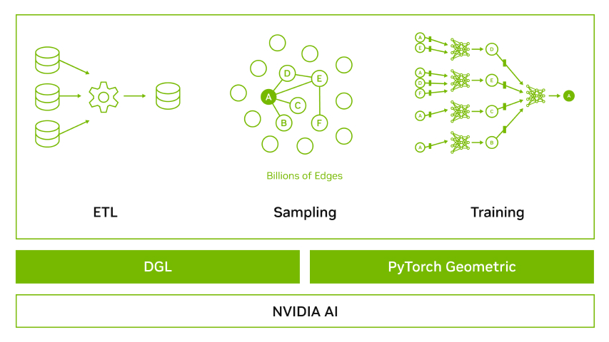
To enable developers to quickly take advantage of GNNs to optimize and accelerate fraud detection, NVIDIA partnered with the Deep Graph Library (DGL) team and the PyTorch Geometric (PyG) team to provide a GNN framework containerized solution that includes the latest DGL or PyG, PyTorch, NVIDIA RAPIDS, and a set of tested dependencies. The NVIDIA-optimized GNN Framework containers are performance-tuned and tested for NVIDIA GPUs. 

This approach eliminates the need to manage packages and dependencies or build the framework from source. We are actively contributing to enhance the performance of these top GNN frameworks. We have added GPU support for unified virtual addressing (UVA), FP16 operations, neighborhood sampling, subgraph operations for minibatches and optimized sparse embeddings, sparse adam optimizer, graph batching, CSR-to-COO conversions, and much more.

This post first addresses the unique problems in credit card fraud detection and the most widely used detection techniques. It also highlights how GNNs accelerated by GPUs have a unique approach to addressing these issues. We walk through an end-to-end workflow showcasing best practices for preprocessing, training, and deployment for detecting fraud on a financial fraud dataset using graph neural networks. Last, we show benchmarks of end-to-end workflows on two industry scale datasets utilizing the optimizations contributed in DGL by NVIDIA engineers.

Overview of fraud detection

Fraud detection is a set of processes and analyses that allow firms to identify and prevent unauthorized activity. It has become one of the major challenges for most organizations, particularly those in banking, finance, retail, and e-commerce. 

Any kind of fraud negatively affects an organization’s bottom line and market reputation, and deters both future prospects and current customers. Given the scale and reach of these vulnerable organizations, it has become crucial for them to prevent fraud from happening and even predict suspicious actions in real time.

Fraud detection poses unique problems for machine learning researchers and engineers, a few of which are detailed below.

Complex and evolving fraud patterns 

Fraudsters update their knowledge and develop sophisticated techniques to cheat the system, often involving complex chains of transactions to avoid detection. 

Traditional ruled-based systems and tabular machine learning (ML) like SVMs and XGBoost often can only consider the immediate edges of a transaction (who sent money to who), often missing patterns of fraud with more complex context. Rule-based systems also need to be hand-tuned over time as patterns of fraud change and new exploits emerge.

Label quality

Available fraud datasets are often both imbalanced and without exhaustive labels. In the real world, only a small percentage of people intend to commit fraud. Domain experts typically classify transactions as either fraudulent or not, but cannot guarantee that all fraud has been captured in the dataset. 

This class imbalance and lack of exhaustive labels make it difficult to develop supervised models, as models trained on the labels we do have may incur higher rates of false negatives, and the imbalanced dataset can lead to models that also generate more false positives. Thus, training GNNs with alternative objectives and using their latent representations downstream can have beneficial effects.

Model explainability 

Predicting whether a transaction is fraudulent or not is not sufficient for transparency expectations in the financial services industry. It is also necessary to understand why certain transactions are flagged as fraud. This explanabity is important for understanding how fraud happens, how to implement policies to reduce fraud, and to make sure the process isn’t biased. Therefore, fraud detection models are required to be interpretable and explainable which limits the selection of models that analysts can use. 

Graph approaches for fraud detection

A series of transactions can be accurately described as a graph, with users being represented as nodes, and transactions between them being represented as edges. While feature-based algorithms like XGBoost and deep feature-based models like DLRM focus on the features of a single node or edge, graph-based approaches can take the features and structure of the local graph context (neighbors and neighbors of neighbors, for example) into account in their predictions.

In the traditional (non-GNN) graph domain, there are many approaches to generating salient predictions based on the graph structure. Statistical approaches that aggregate features from adjacent neighboring nodes or edges, or even their neighbors, can be used to provide information about locality to feature-based tabular algorithms like XGBoost. 

Algorithms like the Louvain method and InfoMap can detect communities and denser clusters of users on the graph, which can then be used to detect communities and generate features that represent graph structure as a hierarchy.

While these approaches can generate adequate results, the problem remains that the algorithms used lack expressivity with respect to the graph itself, as they do not consider the graph in its native format.

Graph neural networks build on the concept of representing local structural and feature context natively within the model. Information from both edge and node features is propagated through aggregation and message passing to neighboring nodes. 

When multiple layers of graph convolution are performed, this results in a node’s state containing some information from nodes multiple layers away, effectively allowing the GNN to have a “receptive field” of nodes or edges multiple jumps away from the node or edge in question. 

In the context of the fraud detection problem, this large receptive field of GNNs can account for more complex or longer chains of transactions that fraudsters can use for obfuscation. Additionally, changing patterns can be accounted for by iterative retraining of the model.

Graph neural networks also benefit from being able to encode meaningful representations of nodes or edges while training on an unsupervised or self-supervised task, such as Bootstrapped Graph Latents (BGRL) or link prediction with negative sampling. This allows GNN users to pre-train a model without labels, and to fine-tune the model on the much sparser labels later in the pipeline, or to output strong representations of the graph. The representation output can be used for downstream models like XGBoost, other GNNs, or clustering techniques.

GNNs also have a suite of tools to enable explainability with respect to the input graph. Certain GNN models like heterogeneous graph transformer (HGT) and graph attention network (GAT) enable an attention mechanism across the adjacent edges of a node at each layer of the GNN, allowing the user to identify the path of messages that the GNN is using to derive its final state. Even if GNN models have no attention mechanism, a variety of approaches have been proposed in order to explain GNN output in the context of the entire subgraph, including GNNExplainer, PGExplainer, and GraphMask.

The next section walks through an end-to-end credit card fraud detection workflow. This workflow uses TabFormer, a card transaction fraud dataset, and trains a R-GCN (relational graph convolutional network) model on a variation of the link prediction task in order to generate enriched node embeddings. These node embeddings are passed to a downstream XGBoost model which is trained and subsequently performs fraud detection. 

This XGBoost model can then be easily deployed. The embeddings trained can subsequently be used for other unsupervised techniques like clustering to identify undiscovered patterns of use without needing labels. Last, we will show benchmarks of end-to-end workflows on two industry scale datasets utilizing the optimizations contributed in DGL by NVIDIA engineers.

Building an end-to-end fraud detection workflow with GNNs

Data preprocessing

We are using the Tabformer dataset provided by IBM to demonstrate this workflow. The TabFormer dataset is a synthetic close approximation of a real-world financial fraud-detection dataset, consisting of:

• 24 million unique transactions
• 6,000 unique merchants
• 100,000 unique cards
• 30,000 fraudulent samples (0.1% of total transactions)

To begin, preprocess the dataset using a predefined workflow. The workflow leverages cuDF, a GPU DataFrame library, to perform feature transformations on the original dataset to prepare it for graph construction. cuDF is a drop in replacement of pandas that enables the preprocessing of data directly on GPUs. 

In this dataset, the card_id is defined as one card by one user. A specific user can have multiple cards, which would correspond to multiple different card_ids for this graph. The merchant_id is the categorical encoding of the feature, ‘Merchant Name’. The data is split such that the training data is all transactions before the year 2018, the validation data is all transactions during the year 2018, and the test data is all transactions after the year 2018. 

# Read the dataset
data = cudf.read_csv(self.source_path)
data[“card_id”] = data[“user”].astype(“str”) + data[“card”].astype(“str”)

# Split the data based on the year
data["split"] = cudf.Series(np.zeros(data["year"].size), dtype=np.int8)
data.loc[data["year"] == 2018, "split"] = 1
data.loc[data["year"] > 2018, "split"] = 2
train_card_id = data.loc[data["split"] == 0, "card_id"]
train_merch_id = data.loc[data["split"] == 0, "merchant_id"]

Strip the ‘$’ from the ‘Amount’ to cast that value as a float. Keep card_id and merchant_id in the validation and test datasets only if they are included in the train datasets.  

The graph is constructed with transaction edges between card_id and merchant_id.

Further preprocessing includes one hot encoding the Use chip feature, label encoding the ‘Is Fraud?’ feature, and target encoding the categorical representations of Merchant State, Merchant City, Zip, and MCC. In addition, the possible values of ‘Errors?’ are one hot encoded.

# Target encoding
high_card_cols = ["merchant_city", "merchant_state", "zip", "mcc"]
for col in high_card_cols:
    tgt_encoder = TargetEncoder(smooth=0.001)
    train_df[col] = tgt_encoder.fit_transform(
        train_df[col], train_df["is_fraud"])
    valtest_df[col] = tgt_encoder.transform(valtest_df[col])

# One hot encoding `use_chip`
oneh_enc_cols = ["use_chip"]
data = cudf.concat([data, cudf.get_dummies(data[oneh_enc_cols])], axis=1)

# Label encoding `is_fraud`
label_encoder = LabelEncoder()
train_df["is_fraud"] = label_encoder.fit_transform(train_df["is_fraud"])
valtest_df["is_fraud"] = label_encoder.transform(valtest_df["is_fraud"])

# One hot encoding the errors
exploded = data["errors"].str.strip(",").str.split(",").explode()
raw_one_hot = cudf.get_dummies(exploded, columns=["errors"])
errs = raw_one_hot.groupby(raw_one_hot.index).sum()

Once the dataset is preprocessed, transform the tabular format of the dataset into a graph.

Modeling tabular data as a graph

Transforming a table (or multiple tables) into a graph centers around mapping the existing table(s) into the edges, nodes, and features for both structures. In the case of this dataset, we begin by using the transaction table to create edges between the cards and the merchants. In contemporary GNN frameworks, graph edges are represented at a basic level by pairs of node IDs. Nodes are implicit based on the IDs included in the edge lists.

# Defining node type
for ntype in ["card", "merchant"]:
   node_type = {MetadataKeys.NAME: ntype, MetadataKeys.FEAT: []}
   self.node_types.append(node_type)

# Adding attributes of edge data
self.edge_data = dict()
self.edge_data["transaction"] = cudf.DataFrame({
  MetadataKeys.SRC_ID: data["card_id"],
  MetadataKeys.DST_ID: data["merchant_id"],})

# Defining features
features = []
for key in data.keys():
  if key not in ["card_id", "merchant_id"]:
    self.edge_data["transaction"][key] = data[key]
      feat = {
       MetadataKeys.NAME: key,
       MetadataKeys.DTYPE: str(self.edge_data["transaction"][key].dtype),
       MetadataKeys.SHAPE: self.edge_data["transaction"][key].shape,}
      if key in ["is_fraud"]:
        feat[MetadataKeys.LABEL] = True
      features.append(feat)

With the base graph created, it’s time to add the transaction features onto the edges in the graph. Note that in this case, the transaction data is only edge-specific, so the output graph has no node features.

Once the graph is created and populated with features, the model can be applied to it. 

Training the GNN model

Given the label imbalance and imperfect labeling of the dataset, we elected to use an unsupervised task, link prediction, to train the model to create meaningful representations of the nodes. The objective of link prediction is to predict the probability that an edge exists between two nodes. In financial services, this is translated to predicting the probability that a transaction exists between an individual and a merchant. 

Some target nodes within the batch are true edges, which are actual edges that exist in the graph, while others, generated by a negative sampler, are negative edges that do not truly exist. Negative edges are necessary in this case because our training task is the classification between real and fake. There are a variety of proposed ways in which to generate negative edges, but simply uniformly sampling the nodes to get the node endpoints is widely employed and achieves good results. While it is possible to negatively sample actual edges with this approach, most graphs are sparse enough that the probability of this is almost negligible.

Since most transaction graphs are too large to represent in GPU memory, we need to employ a subsampling technique in order to generate smaller localities for our graph to process. Sampling is usually done in two phases in DGL. 

First, perform seed sampling in order to identify the edges or nodes targeted for the GNN to predict on. Next, perform block sampling, also known as neighborhood sampling, to generate the subgraphs surrounding the seeds to use as input to the GNN.

The graph contains edges and nodes that could leak future information from the test set, so we must create an individual data loader and sampling routine for our train, validation, and test sets. The train dataloader is moderately simple, utilizing just edges in the training set for seed sampling, and the train set graph for block sampling. 

For the validation data loader, use the validation edges for seed sampling, but use only the training set graph for block sampling in order to prevent the leakage of information. Apply the same idea to the test set, where the test edges are used for seed sampling and the graph defined by the union of the training and validation sets for block sampling.

In order to accelerate dataloading, use a feature called Universal Virtual Addressing (UVA), which allows us to instantiate our graph such that it can be directly accessed by all the GPUs instead of through the host. When the graph is highly featured, UVA can increase model throughput by a factor of up to 5x.

With data loaders defined and the graph built, instantiate the R-GCN model. Graph convolutional networks are known for encoding features from structured neighborhoods, assigning the same weight to edges connected to the source node. R-GCN builds on top of this and provides relation-specific transformations that depend on the type and direction of an edge. 

The edge’s type information supplements the message calculated for each node. Node’s features and edge’s type are passed as input to the R-GCN model which are transformed into an embedding. R-GCN layers can extract high-level node representations by message passing and graph convolutions.

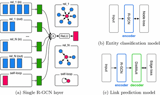
Begin by creating a learnable node-level embedding that stores a 64-element representation tensor for each node. Given that it cannot be used (negative edges are featureless) and the graph has no node features, the node embeddings here will serve as numerical features on nodes in addition to the pure structure of the graph. This embedding table is used as input to the model R-GCN, which is defined using standardized hyperparameters. 

The specified model output is of width 64. Note that this number is not reflective of a number of classes: using link prediction, the R-GCN model should generate a node representation that can be used by a downstream operation to predict the probability of an edge between two nodes. There are many proposed ways to do this, including multi-layer perceptrons. This example uses the cosine similarity of the two nodes in order to generate the probability that nodes are actually connected by an edge. Thus, the model is wrapped in a link predictor module to output probabilities given input representations.

Next, define the optimizers, one for each the model itself and the embedding table. This two-optimizer setup is common within other contexts involving embedding tables, and is used to some effect here in improving model convergence.

With the components defined, it is now time to train the model. Not unlike other domains, the model can be trained on a single node using distributed data parallel (DDP) to further accelerate the model on multiple GPUs.

Using GNN embeddings for downstream tasks

Once the R-GCN model has been trained, generate robust node embeddings using the network. To do this, perform graph convolution at a one-hop scale for each of the graph layers for the entire graph, and use the late-stage activations generated by the model as embeddings of the nodes of the graph.

With the node embeddings generated, join the embeddings onto the original preprocessed dataset on the respective node IDs. Next, fit an XGBoost model to the edge feature dataset augmented with the extracted embedding values from the upstream GNN model. 

First, create a Dask client by connecting to the LocalCUDACluster, which is a Dask based CUDA cluster capable of executing Python processes on multiple GPUs. Then the edge feature dataset is read into Dask and sampled such that the size of the final training dataset, which is defined as edge features augmented with embedding values, does not exceed 40% of the total GPU storage. This is necessary for Dask XGBoost as the full train data must be on GPU memory and the process of creating the DMatrix consumes the rest of the memory. 

Next, the embeddings from the upstream model are read and the node features are appended to its corresponding ID. Finally the XGBoost model is trained to predict ‘Is Fraud?’ and it outputs the AUPRC score of 0.9 on the test set. To demonstrate the efficacy of the GNN-created node embeddings, the best XGBoost model trained on the transactions without them achieves an AUCPR score of 0.79 on the test set.

The model checkpoints can further be used to deploy this model on NVIDIA Triton Inference Server.

Deployment

Once the XGBoost model has been trained, deploy the model and spin up an inference server using a Python backend to handle embedding lookup, and a Forest Inference Library (FIL) backend to perform GPU-accelerated forest library inference. 

The deployment pipeline comprises three parts:

• A Python backend model, referred to as the embedding model. It reads in the embedding tensors. This backend accepts the card IDs and merchant IDs as input and returns their embeddings.
• A FIL backend model, referred to as the XGBoost model. It loads in the saved XGB model from training. This backend accepts the augmented data (features plus embeddings) and returns the XGB prediction for each row.
• Another Python backend model which we refer to as the downstream model. This model unifies the full deployment. This backend accepts the card IDs, merchant IDs, and the features. First it calls the embedding model using business logic scripting (BLS) to get the embeddings. Next, it joins the features and embeddings to create the augmented data. It then calls the XGB model, again using BLS, and returns its predictions.

Query this service with a data sample to get the probability of the transaction being fraudulent. This probability can then be used for developing subsequent business logic.

Benchmarks

We have performed extensive tests on one fraud detection and one benchmark dataset: TabFormer and MAG240M, respectively. To make our experiments reproducible, we have used DGX A100 (80 GB) for all the benchmark runs. This server has 64 core, dual socket AMD EPYC 7742 CPU processors and eight NVIDIA A100 (80 GB SXM4) GPU processors.

The next section presents the speedup achieved by optimizing the end-to-end workflow for GPUs.

TabFormer dataset

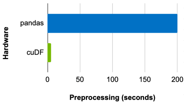
Comparing the time it takes to preprocess the dataset using pandas on a CPU and cuDF on a GPU shows a batch size of 8,192 achieves a 39x speedup with GPU (Figure 2).

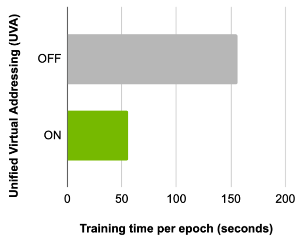
Next, comparing the training time per epoch, before and after enabling this feature, shows the advantages of using UVA. With the same batch size and a fanout of [5, 5] configuration, a 2.8x speedup is achieved on a single GPU (Figure 3).

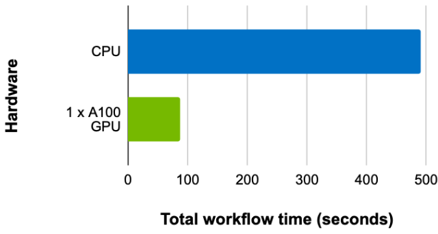
Finally, comparing the training time with the same batch size and fanout configuration, but on a CPU and a GPU (with UVA on) shows a speedup of 5.63x on a single GPU (Figure 4).

MAG240M dataset

The MAG240M dataset is a part of the OGB Large Scale Challenge. It is the largest public benchmark dataset for node-level tasks with ~245 million nodes and ~1.7 billion edges.

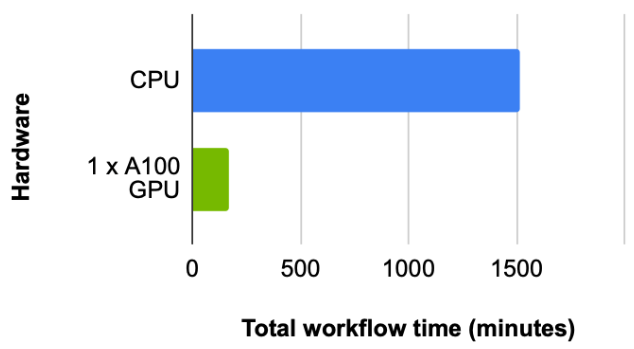
For this dataset, we first look at the total workflow time (the time it takes to preprocess the data), load, plus construct the graph and train the RGCN model. With a batch size of 4,096 and fanout of [150, 100] (used to achieve best results in hyperparameter search), we observe a ~9x speedup where the CPU takes 1,514 minutes and 1x NVIDIA A100 GPU takes 169 minutes (Figure 5).

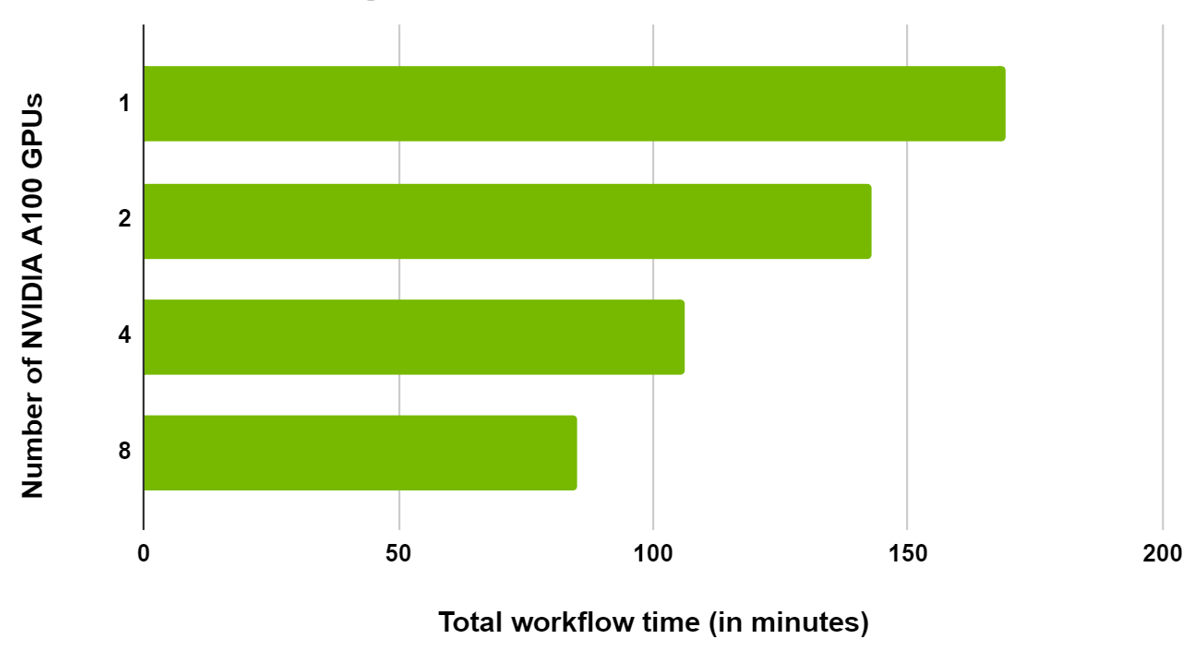
As this is a large dataset, the workflow has been scaled across multiple GPUs in the same node. We observed a 20% reduction in total time when scaling from one to two GPUs and a 50% reduction from one to eight GPUs (Figure 6).

Summary

NVIDIA has partnered with DGL and PyG to add support for graph operations on GPU and optimize preprocessing and training operations. Learn more about how NVIDIA is actively contributing to enhance these top GNN frameworks.

This post has presented an end-to-end workflow of fraud detection with GNNs including preprocessing, modeling tabular data as graph, training GNN, using GNN embeddings for downstream tasks, and deployment. This approach makes use of the NVIDIA optimized DGL, with a set of dependencies like RAPIDS cuDF and NVIDIA Triton Inference Server. We further demonstrated benchmarks on two datasets wherein we observed a 29x speedup of RGCN on MAG240M dataset on one NVIDIA A100 GPU versus CPU.

To learn more, watch the GTC session, Accelerate and Scale GNNs with Deep Graph Library and GPUs with Da Zheng, a senior applied scientist at AWS. See also Accelerating GNNs with Deep Graph Library and GPUs and Accelerating GNNs with PyTorch Geometric and GPUs, hosted by NVIDIA engineers. 

If you have DGL early access or PyG early access, you can now try containers that are performance-tuned and tested for NVIDIA GPUs.