Accelerated Molecular Simulation Using Deep Potential Workflow with NGC

Molecular simulation communities have faced the accuracy-versus-efficiency dilemma in modeling the potential energy surface and interatomic forces for decades. Deep Potential, the artificial neural network force field, solves this problem by combining the speed of classical molecular dynamics (MD) simulation with the accuracy of density functional theory (DFT) calculation.¹ This is achieved by using the GPU-optimized package DeePMD-kit, which is a deep learning package for many-body potential energy representation and MD simulation.²

This post provides an end-to-end demonstration of training a neural network potential for the 2D material graphene and using it to drive MD simulation in the open-source platform Large-scale Atomic/Molecular Massively Parallel Simulator (LAMMPS).³ Training data can be obtained either from the Vienna Ab initio Simulation Package (VASP)⁴, or Quantum ESPRESSO (QE).⁵

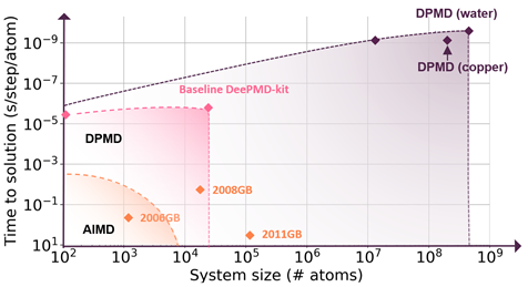
A seamless integration of molecular modeling, machine learning, and high-performance computing (HPC) is demonstrated with the combined efficiency of molecular dynamics with ab initio accuracy — that is entirely driven through a container-based workflow. Using AI techniques to fit the interatomic forces generated by DFT, the accessible time and size scales can be boosted several orders of magnitude with linear scaling.

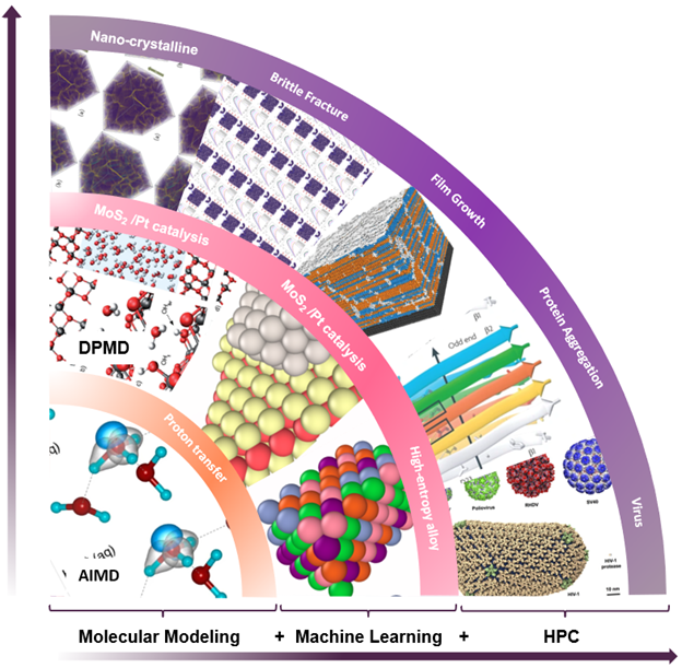
Deep potential is essentially a combination of machine learning and physical principles, which start a new computing paradigm as shown in Figure 1.

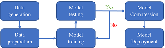
The image shows the new computing paradigm that combines molecular modeling, machine learning and high-performance computing to understand the interatomic forces of molecules compared to the traditional methods. — *Figure 1. A new computing paradigm composed of molecular modeling, AI, and HPC. (Figure courtesy: Dr. Linfeng Zhang, DP Technology)*

The entire workflow is shown in Figure 2. The data generation step is done with VASP and QE. The data preparation, model training, testing, and compression steps are done using DeePMD-kit. The model deployment is in LAMMPS.

This figure displays the workflow of training and deploying a deep potential model. The workflow includes data generation, data preparation, model training, model testing, model compression, and model deployment. — *Figure 2. Diagram of the DeePMD workflow.*

Why Containers?

A container is a portable unit of software that combines the application, and all its dependencies, into a single package that is agnostic to the underlying host OS.

The workflow in this post involves AIMD, DP training, and LAMMPS MD simulation. It is nontrivial and time-consuming to install each software package from source with the correct setup of compiler, MPI, GPU library, and optimization flags.

Containers solve this problem by providing a highly optimized GPU-enabled computing environment for each step, and eliminates the time to install and test software.

The NGC catalog, a hub of GPU-optimized HPC and AI software, carries a whole of HPC and AI containers that can be readily deployed on any GPU system. The HPC and AI containers from the NGC catalog are updated frequently and are tested for reliability and performance — necessary to speed up the time to solution.

These containers are also scanned for Common Vulnerabilities and Exposure (CVEs), ensuring that they are devoid of any open ports and malware. Additionally, the HPC containers support both Docker and Singularity runtimes, and can be deployed on multi-GPU and multinode systems running in the cloud or on-premises.

Training data generation

The first step in the simulation is data generation. We will show you how you can use VASP and Quantum ESPRESSO to run AIMD simulations and generate training datasets for DeePMD. All input files can be downloaded from the GitHub repository using the following command:

git clone https://github.com/deepmodeling/SC21_DP_Tutorial.git

VASP

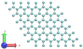
A two-dimensional graphene system with 98-atoms is used as shown in Figure 3.⁶ To generate the training datasets, 0.5ps NVT AIMD simulation at 300 K is performed. The time step chosen is 0.5fs. The DP model is created using 1000 time steps from a 0.5ps MD trajectory at a fixed temperature.

Due to the short simulation time, the training dataset contains consecutive system snapshots, which are highly correlated. Generally, the training dataset should be sampled from uncorrelated snapshots with various system conditions and configurations. For this example, we used a simplified training data scheme. For production DP training, using DP-GEN is recommended to utilize the concurrent learning scheme to efficiently explore more combinations of conditions.⁷

The projector-augmented wave pseudopotentials are employed to describe the interactions between the valence electrons and frozen cores. The generalized gradient approximation exchange−correlation functional of Perdew−Burke−Ernzerhof. Only the Γ-point was used for k-space sampling in all systems.

This figure displays the top view of a single layer graphene system with 98 carbon atoms. — *Figure 3. A graphene system composed of 98 carbon atoms is used in AIMD simulation.*

Quantum Espresso

The AIMD simulation can also be carried out using Quantum ESPRESSO, available as a container from the NGC Catalog. Quantum ESPRESSO is an integrated suite of open-source computer codes for electronic-structure calculations and materials modeling at the nanoscale based on density-functional theory, plane waves, and pseudopotentials. The same graphene structure is used in the QE calculations. The following command can be used to start the AIMD simulation:

$ singularity exec --nv docker://nvcr.io/hpc/quantum_espresso:qe-6.8 cp.x < c.md98.cp.in

Training data preparation

Once the training data is obtained from AIMD simulation, we want to convert its format using dpdata so that it can be used as input to the deep neural network. The dpdata package is a format conversion toolkit between AIMD, classical MD, and DeePMD-kit.

You can use the convenient tool dpdata to convert data directly from the output of first-principles packages to the DeePMD-kit format. For deep potential training, the following information of a physical system has to be provided: atom type, box boundary, coordinate, force, viral, and system energy.

A snapshot, or a frame of the system, contains all these data points for all atoms at one-time step, which can be stored in two formats, that is raw and npy.

The first format raw is plain text with all information in one file, and each line of the file represents a snapshot. Different system information is stored in different files named as box.raw, coord.raw, force.raw, energy.raw, and virial.raw. We recommended you follow these naming conventions when preparing the training files.

An example of force.raw:

$ cat force.raw
-0.724  2.039 -0.951  0.841 -0.464  0.363
 6.737  1.554 -5.587 -2.803  0.062  2.222
-1.968 -0.163  1.020 -0.225 -0.789  0.343

This force.raw contains three frames, with each frame having the forces of two atoms, resulting in three lines and six columns. Each line provides all three force components of two atoms in one frame. The first three numbers are the three force components of the first atom, while the next three numbers are the force components of the second atom.

The coordinate file coord.raw is organized similarly. In box.raw, the nine components of the box vectors should be provided on each line. In virial.raw, the nine components of the virial tensor should be provided on each line in the order XX XY XZ YX YY YZ ZX ZY ZZ. The number of lines of all raw files should be identical. We assume that the atom types do not change in all frames. It is provided by type.raw, which has one line with the types of atoms written one by one.

The atom types should be integers. For example, the type.raw of a system that has two atoms with zero and one:

$ cat type.raw
0 1

It is not a requirement to convert the data format to raw, but this process should give a sense on the types of data that can be used as inputs to DeePMD-kit for training.

The easiest way to convert the first-principles results to the training data is to save them as numpy binary data.

For VASP output, we have prepared an outcartodata.py script to process the VASP OUTCAR file. By running the commands:


$ cd SC21_DP_Tutorial/AIMD/VASP/
$ singularity exec --nv docker://nvcr.io/hpc/deepmd-kit:v2.0.3 python outcartodata.py
$ mv deepmd_data ../../DP/

For QE output:

$ cd SC21_DP_Tutorial/AIMD/QE/
$ singularity exec --nv docker://nvcr.io/hpc/deepmd-kit:v2.0.3 python logtodata.py
$ mv deepmd_data ../../DP/

A folder called deepmd_data is generated and moved to the training directory. It generates five sets 0/set.000, 1/set.000, 2/set.000, 3/set.000, 4/set.000, with each set containing 200 frames. It is not required to take care of the binary data files in each of the set.* directories. The path containing the set.* folder and type.raw file is called a system. If you want to train a nonperiodic system, an empty nopbc file should be placed under the system directory. box.raw is not necessary as it is a nonperiodic system.

We are going to use three of the five sets for training, one for validating, and the remaining one for testing.

Deep Potential model training

The input of the deep potential model is a descriptor vector containing the system information mentioned previously. The neural network contains several hidden layers with a composition of linear and nonlinear transformations. In this post, a three layer-neural network with 25, 50 and 100 neurons in each layer is used. The target value, or the label, for the neural network to learn is the atomic energies. The training process optimizes the weights and the bias vectors by minimizing the loss function.

The training is initiated by the command where input.json contains the training parameters:

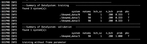
$ singularity exec --nv docker://nvcr.io/hpc/deepmd-kit:v2.0.3 dp train input.json

The DeePMD-kit prints detailed information on the training and validation data sets. The data sets are determined by training_data and validation_data as defined in the training section of the input script. The training dataset is composed of three data systems, while the validation data set is composed of one data system. The number of atoms, batch size, number of batches in the system, and the probability of using the system are all shown in Figure 4. The last column presents if the periodic boundary condition is assumed for the system.

This image is a screenshot of the DP training output. Summaries of the training and validation dataset are shown with detailed information on the number of atoms, batch size, number of batches in the system and the probability of using the system. — *Figure 4. Screenshot of the DP training output.*

During the training, the error of the model is tested every disp_freq training step with the batch used to train the model and with numb_btch batches from the validating data. The training error and validation error are printed correspondingly in the file disp_file (default is lcurve.out). The batch size can be set in the input script by the key batch_size in the corresponding sections for training and validation data set.

An example of the output:

#  step      rmse_val    rmse_trn    rmse_e_val  rmse_e_trn    rmse_f_val  rmse_f_trn         lr
      0      3.33e+01    3.41e+01      1.03e+01    1.03e+01      8.39e-01    8.72e-01    1.0e-03
    100      2.57e+01    2.56e+01      1.87e+00    1.88e+00      8.03e-01    8.02e-01    1.0e-03
    200      2.45e+01    2.56e+01      2.26e-01    2.21e-01      7.73e-01    8.10e-01    1.0e-03
    300      1.62e+01    1.66e+01      5.01e-02    4.46e-02      5.11e-01    5.26e-01    1.0e-03
    400      1.36e+01    1.32e+01      1.07e-02    2.07e-03      4.29e-01    4.19e-01    1.0e-03
    500      1.07e+01    1.05e+01      2.45e-03    4.11e-03      3.38e-01    3.31e-01    1.0e-03

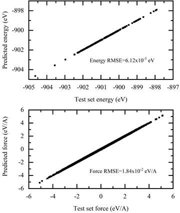
The training error reduces monotonically with training steps as shown in Figure 5. The trained model is tested on the test dataset and compared with the AIMD simulation results. The test command is:

$ singularity exec --nv docker://nvcr.io/hpc/deepmd-kit:v2.0.3 dp test -m frozen_model.pb -s deepmd_data/4/ -n 200 -d detail.out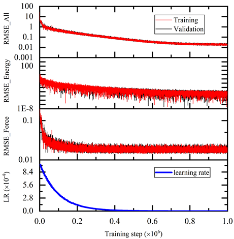

This image shows the total training loss, energy loss, force loss and learning rate decay with training steps from 0 to 1,000,000. Both the training and validation loss decrease monotonically with training steps. — *Figure 5. Training loss with steps*

The results are shown in Figure 6.

This image displays the inferenced energy and force in the y-axis, and the ground true on the x-axis. The inferenced values soundly coincide with the ground truth with all data distributed in the diagonal direction. — *Figure 6. Test of the prediction accuracy of trained DP model with AIMD energies and forces.*

Model export and compression

After the model has been trained, a frozen model is generated for inference in MD simulation. The process of saving neural network from a checkpoint is called “freezing” a model:

$ singularity exec --nv docker://nvcr.io/hpc/deepmd-kit:v2.0.3 dp freeze -o graphene.pb

After the frozen model is generated, the model can be compressed without sacrificing its accuracy; while greatly speeding up the inference performance in MD. Depending on simulation and training setup, model compression can boost performance by 10X, and reduce memory consumption by 20X when running on GPUs.

The frozen model can be compressed using the following command where -i refers to the frozen model and -o points to the output name of the compressed model:

$ singularity exec --nv docker://nvcr.io/hpc/deepmd-kit:v2.0.3 dp compress -i graphene.pb -o graphene-compress.pb

Model deployment in LAMMPS

A new pair-style has been implemented in LAMMPS to deploy the trained neural network in prior steps. For users familiar with the LAMMPS workflow, only minimal changes are needed to switch to deep potential. For instance, a traditional LAMMPS input with Tersoff potential has the following setting for potential setup:

pair_style		tersoff
pair_coeff		* * BNC.tersoff C

To use deep potential, replace previous lines with:

pair_style		deepmd graphene-compress.pb
pair_coeff		* *

The pair_style command in the input file uses the DeePMD model to describe the atomic interactions in the graphene system.

The graphene-compress.pb file represents the frozen and compressed model for inference.
The graphene system in MD simulation contains 1,560 atoms.
Periodic boundary conditions are applied in the lateral x– and y-directions, and free boundary is applied to the z-direction.
The time step is set as 1 fs.
The system is placed under NVT ensemble at temperature 300 K for relaxation, which is consistent with the AIMD setup.

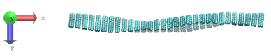
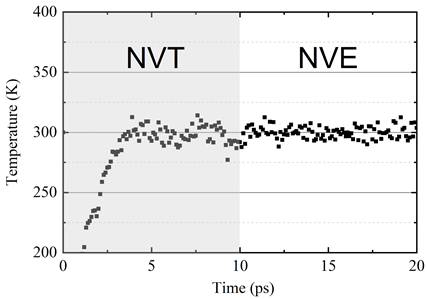
The system configuration after NVT relaxation is shown in Figure 7. It can be observed that the deep potential can describe the atomic structures with small ripples in the cross-plane direction. After 10ps NVT relaxation, the system is placed under NVE ensemble to check system stability.

The image displays the side view of the single layer graphene system after thermal relaxation in LAMMPS. — *Figure 7. Atomic configuration of the graphene system after relaxation with deep potential.*

The system temperature is shown in Figure 8.

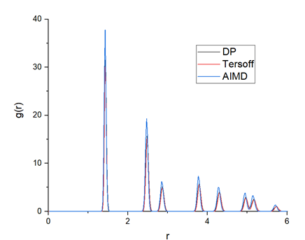
The image displays the temperature profiles of the graphene system under NVT and NVE ensembles from 0 to 20 picoseconds. The first 10 picosecond is NVT and the second 10 picosecond is NVE. — *Figure 8. System temperature under NVT and NVE ensembles. The MD system driven by deep potential is very stable after relaxation.*

To validate the accuracy of the trained DP model, the calculated radial distribution function (RDF) from AIMD, DP and Tersoff, are plotted in Figure 9. The DP model-generated RDF is very close to that of AIMD, which indicates that the crystalline structure of graphene can be well presented by the DP model.

This image displays the plotted radial distribution function from three different methods, including DP, Tersoff and AIMD, which are denoted in black, red and blue solid lines respectively. — *Figure 9. Radial distribution function calculated by AIMD, DP and Tersoff potential, respectively. It can be observed that the RDF calculated by DP is very close to that of AIMD.*

Conclusion

This post demonstrates a simple case study of graphene under given conditions. The DeePMD-kit package streamlines the workflow from AIMD to classical MD with deep potential, providing the following key advantages:

Highly automatic and efficient workflow implemented in the TensorFlow framework.
APIs with popular DFT and MD packages such as VASP, QE, and LAMMPS.
Broad applications in organic molecules, metals, semiconductors, insulators, and more.
Highly efficient code for HPC with MPI and GPU support.
Modularization for easy adoption by other deep learning potential models.

Furthermore, the use of GPU-optimized containers from the NGC catalog simplifies and accelerates the overall workflow by eliminating the steps to install and configure software. To train a comprehensive model for other applications, download the DeepMD Kit Container from the NGC catalog.

Acknowledgements

We thank the helpful discussions with Dr. Chunyi Zhang from Temple University, Dan Han, Dr. Xinyu Wang from Shandong University, and Dr. Linfeng Zhang, Yuzhi Zhang, Jinzhe Zeng, Duo Zhang, and Fengbo Yuan from the DeepModeling community.

References

[1] Jia W, Wang H, Chen M, Lu D, Lin L, Car R, E W and Zhang L 2020 Pushing the limit of molecular dynamics with ab initio accuracy to 100 million atoms with machine learning IEEE Press 5 1-14

[2] Wang H, Zhang L, Han J and E W 2018 DeePMD-kit: A deep learning package for many-body potential energy representation and molecular dynamics Computer Physics Communications 228 178-84

[3] Plimpton S 1995 Fast Parallel Algorithms for Short-Range Molecular Dynamics Journal of Computational Physics 117 1-19

[4] Kresse G and Hafner J 1993 Ab initio molecular dynamics for liquid metals Physical Review B 47 558-61

[5] Giannozzi P, Baroni S, Bonini N, Calandra M, Car R, Cavazzoni C, Ceresoli D, Chiarotti G L, Cococcioni M, Dabo I, Dal Corso A, de Gironcoli S, Fabris S, Fratesi G, Gebauer R, Gerstmann U, Gougoussis C, Kokalj A, Lazzeri M, Martin-Samos L, Marzari N, Mauri F, Mazzarello R, Paolini S, Pasquarello A, Paulatto L, Sbraccia C, Scandolo S, Sclauzero G, Seitsonen A P, Smogunov A, Umari P and Wentzcovitch R M 2009 QUANTUM ESPRESSO: a modular and open-source software project for quantum simulations of materials Journal of Physics: Condensed Matter 21 395502

[6] Humphrey W, Dalke A and Schulten K 1996 VMD: Visual molecular dynamics Journal of Molecular Graphics 14 33-8

[7] Yuzhi Zhang, Haidi Wang, Weijie Chen, Jinzhe Zeng, Linfeng Zhang, Han Wang, and Weinan E, DP-GEN: A concurrent learning platform for the generation of reliable deep learning based potential energy models, Computer Physics Communications, 2020, 107206.