Extracting Features from Multiple Audio Channels with Kaldi

In automatic speech recognition (ASR), one widely used method combines traditional machine learning with deep learning. In ASR flows of this type, audio features are first extracted from the raw audio. Features are then passed into an acoustic model. The acoustic model is a neural net trained on transcribed data to extract phoneme probabilities from the features. A phoneme is a single, distinct vowel or consonant sound. The acoustic model produces a vector of phoneme probabilities based on both the audio data and trained knowledge of the specific language being transcribed. Finally, the phoneme probabilities are passed into a hidden Markov language model, which produces text. For more information about a higher-level view of ASR, see How to Build Domain Specific Automatic Speech Recognition Models on GPUs.

This post describes improvements to the C API for GPU-accelerated feature extraction routines in an ASR package called Kaldi. For more information about making use of GPUs for feature extraction in Kaldi, see Integrating NVIDIA Triton Inference Server with Kaldi ASR.

ASR methods

This post focuses on recent improvements to the first feature extraction step using NVIDIA GPUs. Most methods of feature extraction involve a Fourier transform on many short windows of raw audio to determine the frequency content of these windows. These windows are typically 10-30 milliseconds in length and are called frames. Operations on the frequency spectrum of each frame produce between 10 and 50 features for that frame. The specific operations used to transform the frequency spectrum into features depend on the type of feature extraction and the options selected. Two common feature extraction methods are Mel-frequency cepstral coefficients (MFCC) and filter banks. 

It is often useful in feature extraction to adjust the parameters for the characteristics of individual speakers. Many successful ASR packages use i-vectors both to recognize speakers and to adjust for the pitch, tone, and accent of individuals and the background environment. In feature extraction, speaker characteristics can be either predetermined and passed into the extractor or, more commonly, computed and applied on the fly as features are extracted. In this method, as audio data are processed, the speaker characteristics are refined and immediately applied to the remaining audio.

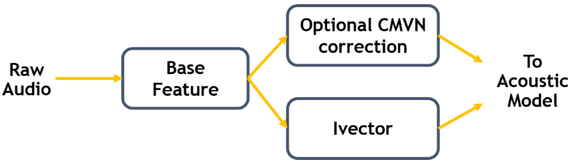
Figure 1 shows that the first step in feature extraction is determination of the base features. Kaldi currently supports GPU feature extraction for either MFCC or filter banks. Following that step, the features can be optionally corrected based on i-vector data or by a cepstral mean and variance normalization (CMVN), which reduces distortion by ensuring each of the individual features have similar statistical characteristics. Both i-vector correction and CMVN are optional.

GPU feature extraction with Kaldi

Some of the challenges for GPU feature extraction are described in the recent GTC session, Speech Recognition Using the GPU Accelerated Kaldi Framework. 

This post highlights some of the features of GPU feature extraction in the open-source Kaldi-ASR package and can help you to set up Kaldi-ASR to make use of your NVIDIA GPUs. The focus of this post is on inference and we do not spend much time discussing ASR model training. However, because feature extraction is not typically trained and is only used to prepare data for the neural network, the feature extraction step for model training is similar.

The Kaldi-ASR package can be downloaded from the kaldi-asr/kaldi GitHub repo. For more information about using the Kaldi Docker container on NGC, see GPU-Accelerated Speech to Text with Kaldi: A Tutorial on Getting Started. To date, GPU processing is supported for MFCC, filter banks, CMVN, and i-vector extraction.

Batched online feature extraction

Previously, GPU feature extraction in Kaldi involved using the whole GPU to process a single audio file from raw audio to transcribed text. All the audio had to be present as feature extraction began. Kaldi has been recently modified to extract features from a few seconds of audio from several hundred channels at the same time. This improves the practicality of Kaldi in two significant ways:

• First, the latency is much improved, especially when real-time audio from multiple sources as processing can begin as soon as audio data is available.
• Second, the throughput of Kaldi is improved due to greater parallelism exposed to the GPU kernels.

The recent GTC session, Accelerate Your Speech Recognition Pipeline on the GPU, details the changes to accommodate online processing, meaning audio is transcribed live before the entire audio file is available. The changes to allow multiple simultaneous channels are described later in this post. The throughput and latency of feature extraction depend on the number of channels processed simultaneously and on the length of the audio segments from each channel. These dependencies are also discussed later.

For batched processing, the concept of “lanes” represents hardware slots for the processing of a single audio source known as a channel. For feature extraction, one channel with new, unprocessed data is assigned to each lane and input data are copied into the appropriate row in the input array before launching the feature extraction routine. 

The Kaldi source code includes an example of the new batched interface. In src/cudafeatbin, the file compute-online-feats-batched-cuda.cc extracts features from audio files using the online, batched flow. This file can be built into a binary that extracts features from a specified list of .wav audio files. The online and batched specifiers indicate that the audio is processed a few seconds at a time, returning features as they are computed, and that several audio files are processed at one time. The binary itself still waits for the whole audio files to be finished before writing out features, but the interface that it demonstrates returns features as each batch finishes.

In that source file, the audio data are first read in and staged to the CPU. For this sample code, all the audio data are read from the files at one time, but the API allows data to be read in as they become available. The ComputeFeaturesBatched interface discussed later expects CPU pointers and handles data movement to the GPU itself.

To launch a batch of audio for processing, it is important to provide a list of work for the GPU. The work list specifies the input data and some flags and metadata describing how many samples are present and whether this is the beginning or the end of an audio file. 

The audio input data and the output data are stored in Kaldi matrices. The kaldi::Matrix class is defined in the \matrix directory of the Kaldi source code. Data on the GPU is stored in CUDA matrices of type CuMatrix defined in the \cu-matrix directory. A CuMatrix array has member functions NumRows and NumCols to return the number of rows and columns in the matrix. For efficient memory access, matrix rows can be padded. To facilitate correct memory references, CuMatrix also has a member function, Stride, to return the stride between subsequent rows in the matrix.

To call the batched feature extraction pipeline, a CuMatrix array is populated with the audio data. Each row of the CuMatrix array contains an audio segment for a unique audio file. A separate array on the CPU specifies the number of valid samples in each audio segment and two Boolean arrays specify whether you are just beginning or have reached the end of an audio file.

With the metadata correctly populated and audio files in the CuMatrix array, a call to ComputeFeaturesBatched processes the raw audio into audio features for each channel. The call to ComputeFeaturesBatched looks like the following code example:

void ComputeFeaturesBatched(int32 num_lanes,
                            const std::vector<int32> &channels,
                            const std::vector<int32> &num_chunk_samples, 
                            const std::vector<int32> &first, 
                            const std::vector<int32> &last,
                            float sample_freq,
                            const CuMatrix<float> &cu_wave_in,
                            CuMatrix<float> *input_features,
                            CuVector<float> *ivector_features,
std::vector<int32> *num_frames_computed);

The arguments are as follows:

• num_lanes—Number of audio channels processed in this batch. It should also match the length of channels, num_chunk_samples, first and last.
• channels—Contains the channel ID for each channel. Remember that audio data from an audio file should always be passed with the same channel ID.
• num_chunk_samples—Contains the number of valid samples in each audio segment.
• first and last—Boolean arrays specifying whether this chunk represents the first or the last of an audio file.
• sample_freq—The sample frequency of the audio.
• cu_wave_in—A CUDA array containing the audio segments with each row containing the audio segment for a single lane.
• cu_feats_out—A pre-allocated CUDA array for the output features.
• ivector_features—A pre-allocated CUDA vector for the i-vector features; and
• num_frames_computed—Pre-allocated and contains the number of frames computed for each channel.

On output, the features are in the pre-allocated cu_feats_out array. Each row of the CuMatrix array contains the features for one frame. For each lane, ComputeBatchedFeatures produces features for max_chunk_frames frames, although some of those frames may be invalid if fewer samples were provided. The maximum number of frames is returned by the GetMaxChunkFrames member function of OnlineBatchedFeatureCudaPipelineCuda, which can be called to determine the size of the cu_feats_out array. Irrespective of the number of valid frames for each channel, the i-th channel always begins on row i*max_chunk_frames (Figure 2).

These features can then be extracted to the appropriate channels and added to the features computed in previous batches.

The stride for the ivector_features array is given by the IvectorDim member function of OnlineBatchedFeaturePipelineCuda. Each row contains the complete i-vector data for a channel.

Performance

The batching of feature extraction dramatically improves performance. For these comparisons, we used a MFCC plus i-vector model. In the studies shown later in this post, we recorded the time to move the audio data to the GPU, feature extraction time, and time to move the feature data back. Latency refers to the time from start until the first set of features become available on the CPU host. RTFx is the real-time factor, which is the ratio of the total seconds of audio to the total feature extraction time.

This first case involves short audio segments. The audio segments for this dataset varied in length from about five to about 15 seconds. There were 2,500 total files to process. In total, there were 22,700 seconds of audio. Figure 3 plots RTFx against the number of lanes. Different colors show varying numbers of samples per batch. The interface allows the number of valid samples in any channel to be specified. Some batches contain less than the full number of valid audio samples from some channels.

The GPU was a V100-SXM2 with PCIe v3 link to an Intel Broadwell CPU. 

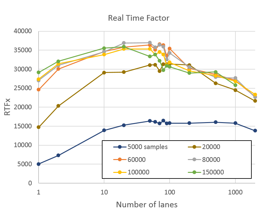
Performance reaches a plateau for nearly all chunk lengths between 30 and 60 channels. Beyond this, the GPU is fully utilized, and tail effects begin to reduce performance. Performance was significantly worse for less than 20,000 samples. Compared with a batch size of one, batched performance is higher by almost 20%.

Figure 4 shows the latency, meaning the time between the start of the GPU computation to the time that the first set of extracted features are available. It rises linearly with the number of batches times the number of samples per chunk. 

Performance improves for longer audio files. The next plot shows the same RTFx measurement for a different dataset. In this dataset, audio files varied in length between 300 and 1,800 seconds. This set had 960 such files for a total length of 967,000 seconds. Figure 5 shows that these longer utterances boost GPU performance. 

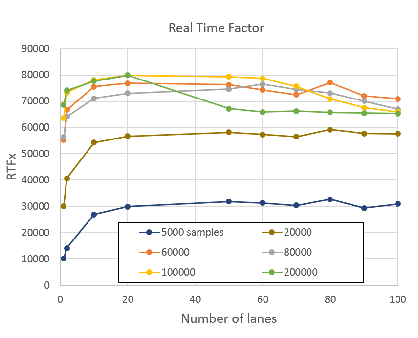
At the peak of 80,000 RTFx, the GPU was able to process the whole 967,000 seconds (eight months!) of audio in 12 seconds.  

As a comparison, feature extraction for the same set using a single core of an E5-2698 v4 Broadwell CPU took 18,300 seconds. If you assume perfect scaling up to the 80 cores of the CPU, the total processing time would be 228 seconds. This is a good assumption as the processing of the 2,500 audio files are independent. This is a 19X speed-up comparing the full GPU with the full CPU.

At peak, the CPU consumes about 120 W, while the V100 consumes 300 W. The performance per watt of the GPU is about 7.6X higher than the 80-core Broadwell CPU.

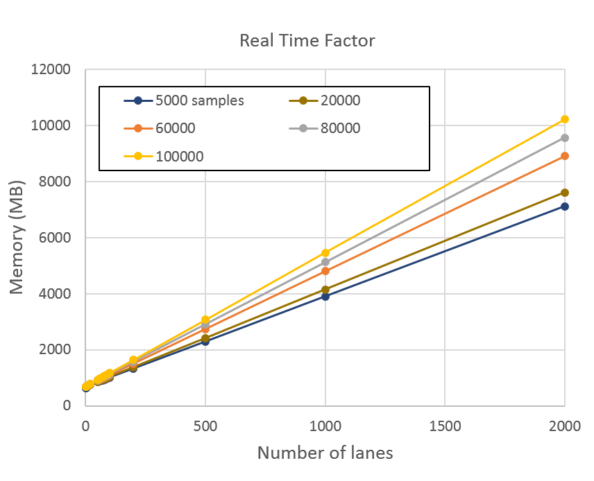
Memory requirements

The CudaOnlineBatchedSpectralFeatures class allocates a few temporary arrays on initialization. Because the audio is processed in chunks, the GPU memory requirements are independent of the length of the audio. The peak GPU memory utilization is plotted in Figure 6 for the same set of chunk size and number of lanes. This experiment is run with the larger, 967,000 second test set and cuda-cache-memory set to false.

Getting started with Kaldi

The batching of real-time audio gives significantly better performance for feature extraction on NVIDIA GPUs. In addition to invoking Kaldi binaries, calls to routines in the open-source Kaldi repository can speed up ASR.

To get started with Kaldi, clone the kaldi-asr/kaldi GitHub repo, which includes GPU support. There are Kaldi-compatible, open-source models for many languages. For more information about accessing and using Kaldi Docker containers from NGC, see NVIDIA Accelerates Real Time Speech to Text Transcription 3500x with Kaldi.