Integrating NVIDIA Triton Inference Server with Kaldi ASR

Speech processing is compute-intensive and requires a powerful and flexible platform to power modern conversational AI applications. It seemed natural to combine the de facto standard platform for automatic speech recognition (ASR), the Kaldi Speech Recognition Toolkit, with the power and flexibility of NVIDIA GPUs.

Kaldi adopted GPU acceleration for training workloads early on. NVIDIA began working with Johns Hopkins University in 2017 to better use GPUs for inference acceleration, by moving all the compute-intensive ASR modules to the GPU. For more information about previous and recent results, see NVIDIA Accelerates Real Time Speech to Text Transcription 3500x with Kaldi and GTC 2020: Accelerate your Online Speech Recognition Pipeline with GPUs.

In this post, we focus on other important improvements to the KALDI ASR pipeline: easy deployment of GPU-powered, low-latency streaming inference with the NVIDIA Triton Inference Server.

Triton Inference Server

Triton Server is an open source inference serving software that lets teams deploy trained AI models from any framework (TensorFlow, TensorRT, PyTorch, ONNX Runtime, or a custom framework), from local storage or Google Cloud Platform or Amazon S3 on any GPU- or CPU-based infrastructure (cloud, data center, or edge). Triton Server provides a cloud inferencing service optimized for NVIDIA GPUs using an HTTP or gRPC endpoint, allowing remote clients to request inferencing for any model being managed by the server.

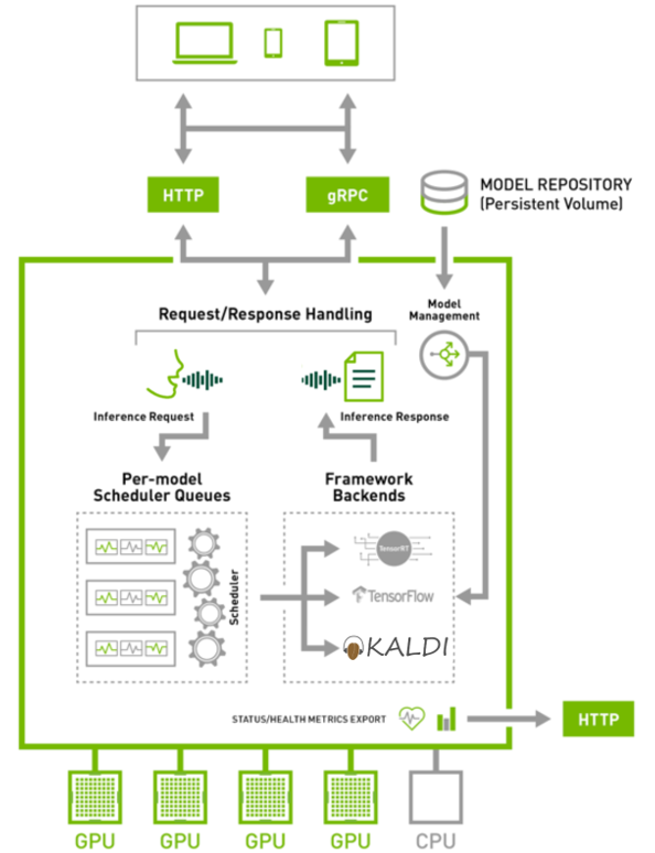
Clients can communicate via HTTP or gRPC with Triton Server represented by a block enclosing a per-model queue scheduler and a multiple framework backends. Triton Server needs access to a model repository and exports metrics through a Rest API. — *Figure. 1. Triton Server block diagram.*

The following features are the most relevant for this post:

Concurrent model execution support: Multiple models, or multiple instances of the same model, can run simultaneously on the same GPU.
Custom backend support: Individual models can be implemented with custom backends instead of a popular framework like TensorFlow or PyTorch. With a custom backend, a model can implement any logic desired, while still benefiting from the GPU support, concurrent execution, dynamic batching, and other features provided by the server.
Multi-GPU support: Triton Server can distribute inferencing across all GPUs in a server.
Dynamic batcher: Inference requests can be combined by the server, so that a batch is created dynamically, resulting in the same increased throughput seen for batched inference requests.
Sequence batcher: Like the dynamic batcher, the sequence batcher combines non-batched inference requests, so that a batch is created dynamically. Unlike the dynamic batcher, the sequence batcher should be used for stateful models where a sequence of inference requests must be routed to the same model instance.

The Kaldi Triton Server integration takes advantage of the sequence batcher. For more information, see the Triton Inference Server User Guide.

Kaldi ASR integration with Triton

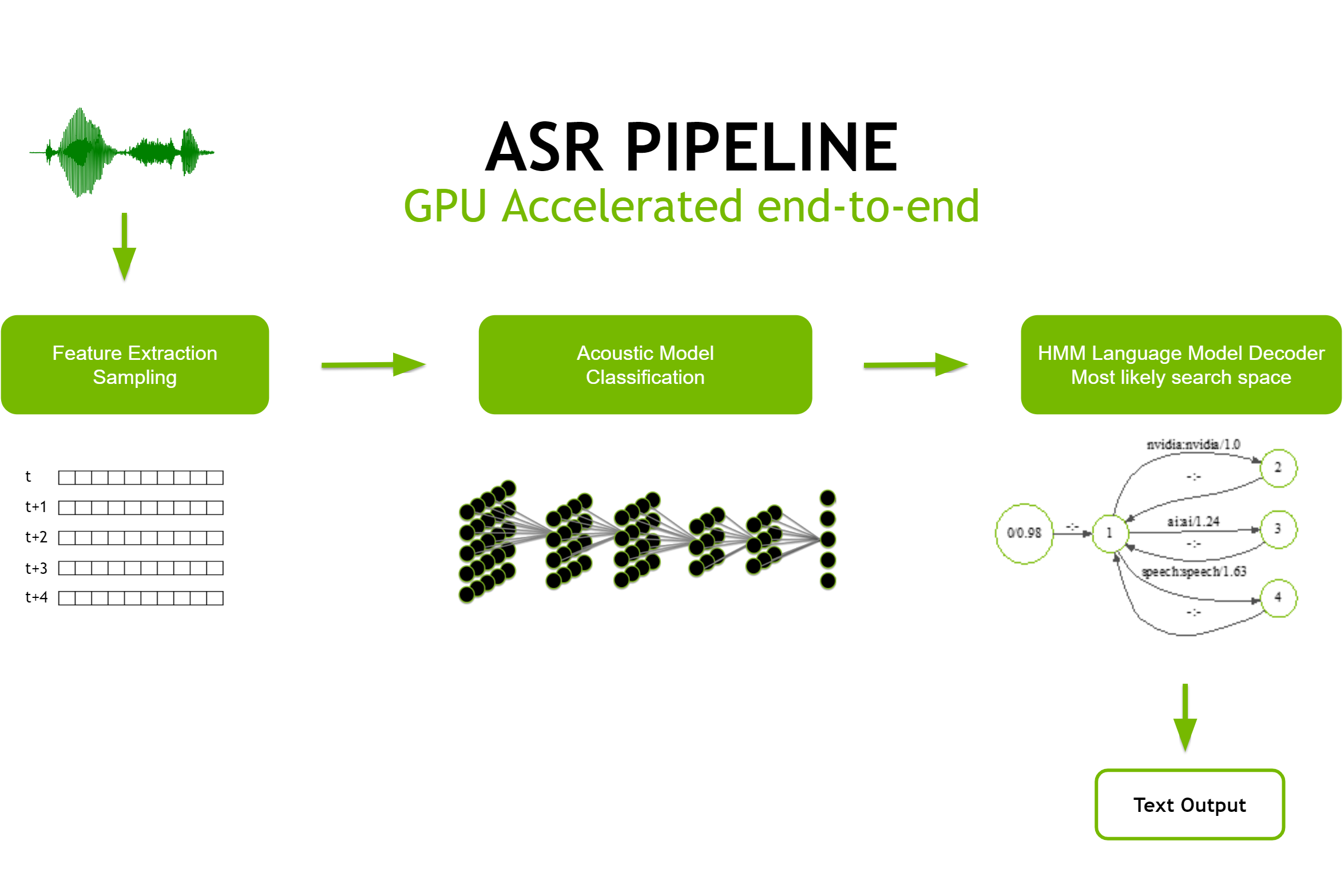
Figure 1 shows a typical pipeline for ASR. The raw input audio containing the utterances is processed to extract features which are sent to an acoustic model for probabilistic classification. Using the likelihoods produced by that classification, and with the help of a language model, you can determine the most likely transcription for that audio.

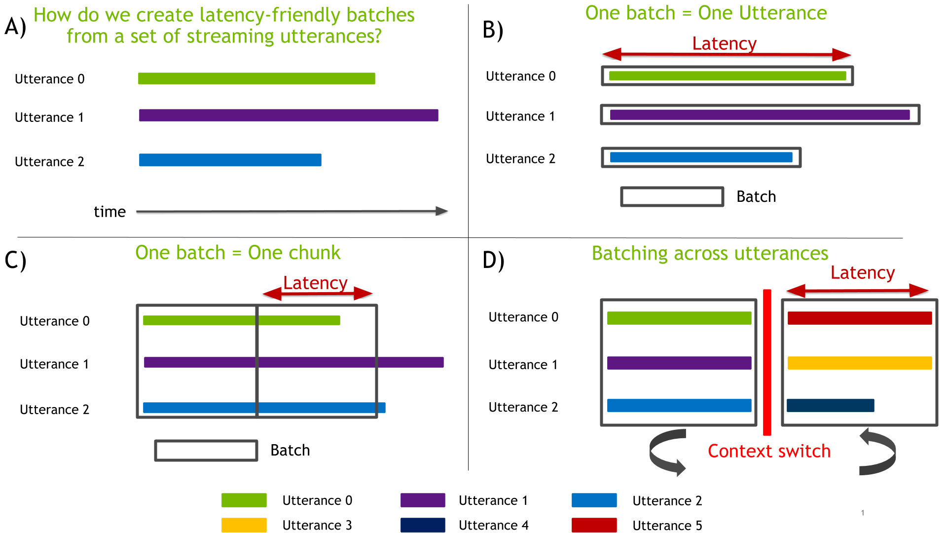
The figure is showing a block diagram representing the ASR pipeline. From the left to the right: A waveform representing the vocal signal is fed to a block for feature extraction, the features obtained are fed to another block representing the acoustic model for classification the output goes into the Language Model Decoder, which in turn returns the transcription of the vocal input. — *Figure 2. The KALDI ASR pipeline implemented as a reference.*

If you wait for the entire utterance to be emitted before streaming the audio, the GPU stays idle until it receives the data (Figure 3, a-b). At this point, a lot of processing needs to happen leading to large latency. To reduce the latency and distribute the load on the GPU more uniformly, you need a better streaming and batch strategy.

An improvement over the earlier scenario is to build bigger batches by streaming multiple utterances emitted by multiple users—0, 1, 2 in Figure 3(c) —at the same time. While you may saturate the GPU in this way, you must still wait for the entire utterance to be produced to generate its transcription. A bigger batch, with even more computation to run, definitely increases latency.

You can further improve this approach by dividing each utterance into small chunks, that can be processed as soon as they are ready. Chunks are typically 100-500ms of audio. At the end of the utterance, you have only the last chunk to process. You end up with a much smaller latency, because you have much less work to do at the very end.

By combining both approaches, you can build large batches using small chunks from multiple utterances, as shown in Figure 3(c).

However, you can compute a batch much faster than that in real time. In the previous scenario, the GPU spends most of its time waiting for the next chunks to be ready. Remove this constraint by implementing multiplexing. Each batch slot is oversubscribed with many audio channels, picking at a given time any channel that is ready to be used.

To do that, you need a fast, on-device context switch. When running inference on multiple sets of utterances, you must restore the previous state of the components, as shown in Figure 3(d). For example, create a first batch with utterances 0, 1, 2 and then a second batch with utterances 3, 4, 5.

The figure is divided into four sub-quadrants. Top-left: multiple utterances happening simultaneously represented by bars of different lengths on a timeline. Top-right: each batch contains a single utterance bar, the latency is therefore at least equal to the length of the utterance. Bottom-left: each batch is obtained by combining chunks from different utterance bars, latency is equal to the last bar chunk. Bottom-right: multiple pools of utterance bars are considered at the same time divided in chunks enclosed in blocks representing context switch between batches. — Figure 3. Multiple utterances happening at the same time (a). Each batch contains a single utterance (b). Each batch is obtained by combining chunks from different utterances (c). Multiple pools of utterances are considered at the same time; this requires a context switch between batches (d).

We have implemented this solution and made it available in the Kaldi ASR framework. This work is based on the online GPU-accelerated ASR pipeline from GPU-Accelerated Viterbi Exact Lattice Decoder for Batched Online and Offline Speech Recognition. The paper included a high-performance implementation of a GPU HMM decoder, a low-latency neural net driver, fast feature extraction for preprocessing, and new ASR pipelines tailored for GPUs.

The integration of the Kaldi ASR framework with Triton Server then added gRPC interface and dynamic batching management for best performance. To download the repository containing the integration of Kaldi with Triton Server, see Kaldi/SpeechRecognition GitHub repo. We included a pretrained version of the Kaldi ASR LibriSpeech recipe for reference model and for demonstration purposes. The LibriSpeech dataset is a large (1,000 hours) corpus of read English speech.

Based on this integration (Figure. 4), a client connects to the gRPC server, streams audio by sending chunks to the server, and gets back the inferred text as an answer. For more information, see Kaldi ASR Quick Start. For testing purposes, this example comes with data for the client to simulate multiple parallel users by streaming multiple audio streams in parallel.

From left to right: Multiple vocal channels are buffered in chunks and sent of the network for dynamic sequence batching. When scheduled the waveform enters the Stateful Feature Extraction, the features obtained are fed in the Stateful Acoustic Model and the Logits Channels finally go to the Stateful HMM Decoder. — Figure 4. A set of channels (vocal assistants), 0…6 in this case, is sending a stream of audio to the server in chunks. The last chunk can be partially filled. From the available channels, you build execution batches and each component (in green) transparently restores the context needed to correctly run inference. The Triton Server integration takes care of the parts in the red boxes and calls the streaming pipeline behind the scenes.

The server expects chunks of audio each containing a fixed but configurable amount of data samples (float array). This is a maximum value, so sending partial chunks is possible. Flags can be set to declare a chunk as a first chunk or last chunk for a sequence. Finally, each chunk from a given sequence is associated with a CorrelationID value. Every chunk belonging to the same sequence must be given the same CorrelationID value. Support for automatic end-pointing will be added in the future.

After the server receives the final chunk for a sequence, with the END flag set, it generates the output associated with that sequence and send it back to the client. The end of the sequencing procedure is as follows:

Process the last chunk.
Flush and process the neural net context.
Generate the full lattice for the sequence.
Determinize the lattice.
Find the best path in the lattice.
Generate the text output for that best path.
Send the text back to the client.

Even if only the best path is used, you are still generating a full lattice for benchmarking purposes. Partial results generated after each timestep are currently not available but will be added in a future release.

Getting started with Kaldi ASR Triton Server

Start by running the server and then the Jupyter notebook client.

Server

Run the Kaldi Triton Server in a Docker container. Install NVIDIA Docker as a prerequisite. For more information about how to get started with NGC containers, see the following:

The first step is to clone the repository:

git clone https://github.com/NVIDIA/DeepLearningExamples.git
cd DeepLearningExamples/Kaldi/SpeechRecognition

Build the client and server containers:

scripts/docker/build.sh

Download and set up the pretrained model and evaluation dataset:

scripts/docker/launch_download.sh

The model and dataset are downloaded in the /data folder.

Start the server:

scripts/docker/launch_server.sh

By default, only GPU 0 is used. Multi-GPU support is planned for future release. Select a different GPU by using NVIDIA_VISIBLE_DEVICES:

NVIDIA_VISIBLE_DEVICES=<GPUID> scripts/docker/launch_server.sh

When you see the line Starting Metrics Service at 0.0.0.0:8002, the server is ready to be used. Start the client.

The following command streams 1000 parallel streams to the server. The -p option prints the inferred text sent back from the server.

scripts/docker/launch_client.sh -p -c 1000

For more information about advanced server configuration, see Kaldi ASR Integration with TensorRT Inference Server.

Client example: Jupyter notebooks

To better show the steps for carrying out inference with the Kaldi Triton backend server we are going to run the JoC/asr_kaldi Jupyter notebooks. You display the results of inference using a Python gRPC client in an offline context, that is with pre-recorded .wav files and in an online context by streaming live audio.

After this step, you should have Triton Server ready to serve ASR inference requests. The next step is to build a Triton Server client container:

docker build -t kaldi_notebook_client -f Dockerfile.notebook .

Start the client container with the following command:

docker run -it --rm --net=host --device /dev/snd:/dev/snd -v $PWD:/Kaldi kaldi_notebook_client

Within the client container, start the Jupyter notebook server:

cd /Kaldi

jupyter notebook --ip=0.0.0.0 --allow-root

Navigate a web browser to the IP address or hostname of the host machine at port 8888:

http://[host machine]:8888

Use the token listed in the output from running the Jupyter command to log in, for example:

http://[host machine]:8888/?token=aae96ae9387cd28151868fee318c3b3581a2d794f3b25c6b

When the Jupyter notebook is running, you can do the following:

Verify the Triton Server status.
Read and preprocess audio files in chunks.
Load data into the server.
Return transcriptions.

Kaldi ASR and Triton Server performance results

To measure performance of the inference server, you stream multiple (1000 or more) parallel streams to the server using the client available with the repository.

To run the performance client, run the following command:

scripts/docker/launch_client.sh -p

The -p option prints the inferred text sent back from the server.

Client command-line parameters

The client can be configured through a set of parameters that define its behavior. To see the full list of available options and their descriptions, use the -h command-line option.

Inference process

Inference is done through simulating concurrent users. Each user is attributed to one utterance from the LibriSpeech dataset. It streams that utterance by cutting it into chunks and gets the final Text output after the final chunk has been sent. A parameter sets the number of active users being simulated in parallel.

Metrics

For the performance of the ASR pipeline, we considered two factors: throughput and latency.

Throughput is measured using the inverse of the real-time factor (RTF) metric: the RTFX metric, which is defined as follows:

$RTFX = \frac{L}{C}$

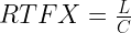
Where L is the length of the input audio in seconds and C is the compute time needed to transcribe it in seconds.

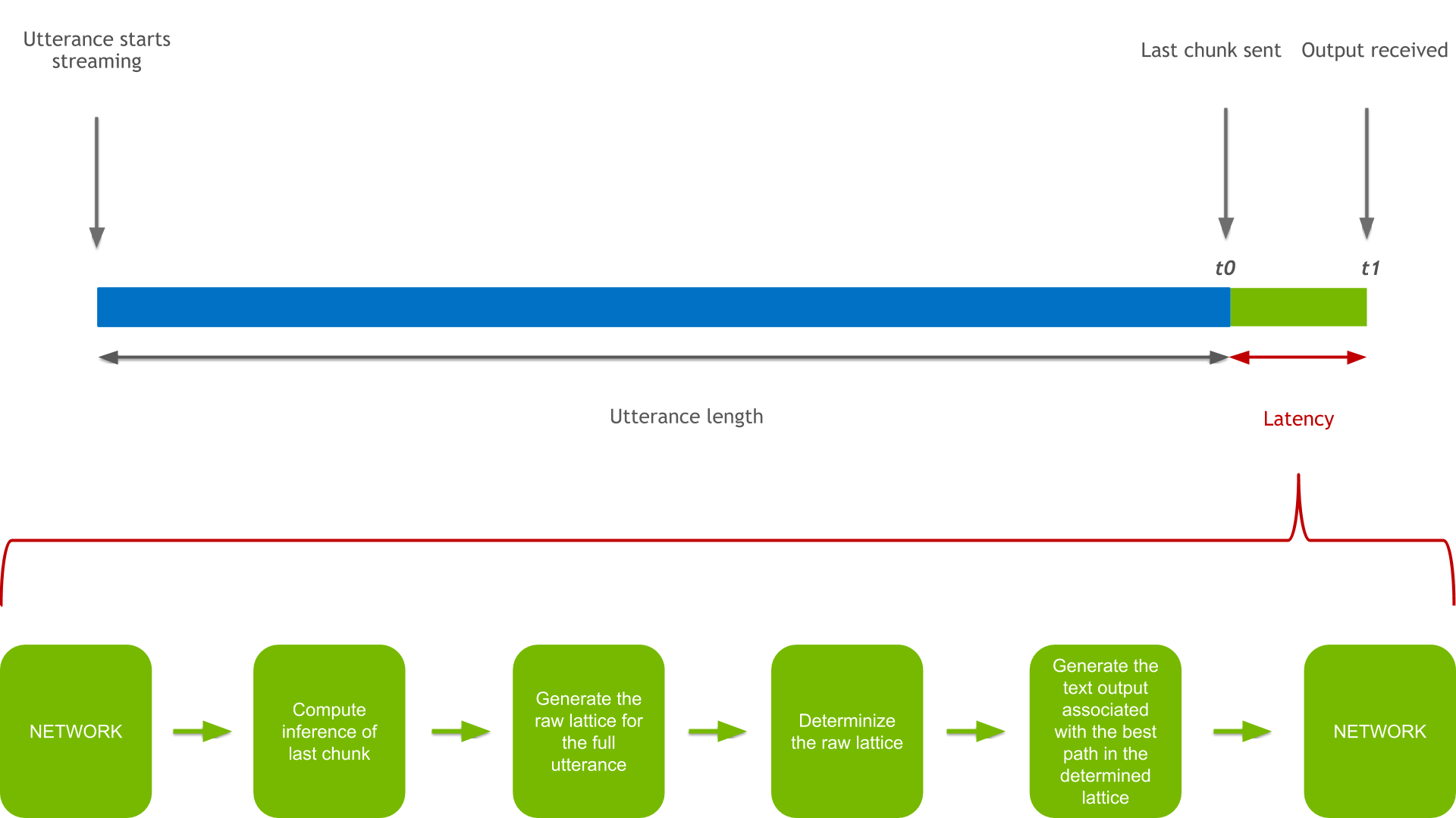
Latency is defined as the delay between the availability of the last chunk of audio and the reception of the transcription. Figure 5 shows the following tasks affecting latency:

Client: Last audio chunk available.
t0 <- Start measuring latency.
Client: Send last audio chunk.
Server: Compute inference of last chunk.
Server: Generate the raw lattice for the full utterance.
Server: Determinize the raw lattice.
Server: Generate the text output associated with the best path in the determined lattice.
Client: Receive text output.
Client: Call callback with output.
t1 <- We stop latency measurement.

So, the latency that you measure is defined as latency = t1 - t0.

: A block diagram that describes the latency from the final chunk of audio available to the received transcription, from left to right: Network, Compute Inference of last chunk, Generate raw lattice for the full utterance, determinizes the raw lattice, generate the text output associated with the best path of the lattice, network. — *Figure 5. Sequence of operation affecting latency from the final chunk of audio available to the received transcription.*

Results

The results were obtained by building and starting the server as described in the Quick Start Guide and running scripts/run_inference_all_v100.sh and scripts/run_inference_all_t4.sh.

Table 1 summarizes the results (RTFX and Latency) obtained for V100 and T4 across different numbers of parallel audio channels.

GPU	Realtime I/O	Number of parallel audio channels	Throughput (RTFX)	Latency (seconds) 90%	Latency (seconds) 95%	Latency (seconds) 99%	Latency (seconds) Avg
V100	No	2000	1506.5	N/A	N/A	N/A	N/A
V100	Yes	1500	1243.2	0.582	0.699	1.04	0.4
V100	Yes	1000	884.1	0.379	0.393	0.788	0.333
V100	Yes	800	660.2	0.334	0.34	0.438	0.288
T4	No	1000	675.2	N/A	N/A	N/A	N/A
T4	Yes	700	629.2	0.945	1.08	1.27	0.645
T4	Yes	400	373.7	0.579	0.624	0.758	0.452

Table 1. Latency and RTFX for V100 and T4 measured using the performance client.

Using a custom Kaldi ASR model

Support for Kaldi ASR models that are different from the provided LibriSpeech model is experimental. However, it is possible to modify the Model Path section of the config file model-repo/kaldi_online/config.pbtxt to set up your own model.

The models and Kaldi allocators are currently not shared between instances. This means that if your model is large, you may end up with not enough memory on the GPU to store two different instances. If that’s the case, you can set count to 1 in the instance_group section of the config file.

Conclusion

In this post, we described the integration between the Kaldi ASR framework and NVIDIA Triton Inference Server. For more information, see the Kaldi/SpeechRecognition GitHub repo.

A Jupyter notebook illustrates how the inference server is expecting requests and how to receive results. We also showed performance results that were obtained by using the performance client included.

Both the Triton Inference Server integration and the underlying Kaldi ASR online GPU pipeline are a work in progress and will support more functionality in the future. This includes online iVectors not currently supported in the Kaldi ASR GPU online pipeline and being replaced by a zero vector. For more information, see Known issues.

Support for a custom Kaldi model is experimental. For more information, see Using a custom Kaldi model.