
DigitalGlobe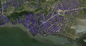 , CosmiQ Works and NVIDIA recently announced the launch of the SpaceNet online satellite imagery repository. This public dataset of high-resolution satellite imagery contains a wealth of geospatial information relevant to many downstream use cases such as infrastructure mapping, land usage classification and human geography estimation. The SpaceNet release is unprecedented: it’s the first public dataset of multi-spectral satellite imagery at such high resolution (50 cm) with building annotations. This information can be used in important applications like real-time mapping for humanitarian crisis response, infrastructure change detection for ensuring high accuracy in the maps used by self-driving cars or figuring out precisely where the world’s population lives. State-of-the-art Artificial Intelligence tools like deep learning show promise for enabling automated extraction of this information with high accuracy.
NVIDIA is proud to support SpaceNet by demonstrating an application of the SpaceNet data that is made possible using GPU-accelerated deep learning.
In this post we demonstrate how DIGITS can be used to train two different types of convolutional neural network for detecting buildings in the SpaceNet 3-band imagery. We hope that this demonstration of automated building detection will inspire other novel applications of deep learning to the SpaceNet data.
SpaceNet Data
The first Area of Interest (AOI) released in the SpaceNet dataset contains two sets of over 7000 images by the DigitalGlobe Worldview-2 satellite over Rio de Janeiro, Brazil. Each image covers 200m2 on the ground and has a pixel resolution of ~50cm. Worldview-2 is sensitive to light in a wide range of wavelengths. 3-band Worldview-2 images are standard natural color images, which means they have three channels containing reflected light intensity in thin spectral bands around the red, green and blue light wavelengths (659, 546 and 478 nanometres (nm) respectively). The 8-band multispectral images contain spectral bands for coastal blue, blue, green, yellow, red, red edge, near infrared 1 (NIR1) and near infrared 2 (NIR2). (corresponding to center wavelengths of 427, 478, 546, 608, 659, 724, 833 and 949 nm, respectively). This extended range of spectral bands allows Worldview-2 8-band imagery to be used to classify the material that is being imaged. For more information on the spectral imaging capabilities of Worldview-2 see [DigitalGlobe 2014]. In this post we will focus solely on the 3-band images. Figure 1 shows two example 3-band images.
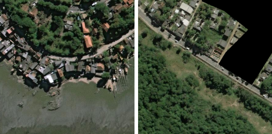
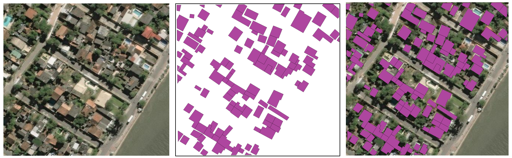
The dataset includes the polygons outlining all building footprints in each image, as Figure 2 shows. Some images contain more than 200 buildings, while others contain none. There are also blank areas in some images that contain no pixel information at all (right-hand side of Figure 1). The dataset shows a variety of different environments, with dense urban areas that have many buildings very close together and sparse rural areas containing buildings partially obstructed by surrounding foliage. Most buildings are quadrilateral but there are more complex building footprints throughout the dataset.
The image data is provided in GeoTIFF format. This is a public domain metadata standard which allows georeferencing information—such as map projections—to be embedded within a TIFF file. This enables precise mapping of each pixel in the image to a location on Earth.
The building footprints are provided in both CSV and GeoJSON formats. The CSV provides the coordinates of the vertices of the building footprint polygons in latitude and longitude in the same map projection as the images, and the GeoJSON provides this same information in pixel coordinates relative to the image.
Building Detection Using DIGITS
There are multiple ways to use DIGITS to detect buildings in satellite images. We will describe two approaches here and show some example results.
Approach 1: Object detection
In an object detection approach we attempt to detect each individual building as a separate object and determine a bounding box around it. Support for object detection was recently added in DIGITS 4. There have been numerous deep learning approaches to object detection proposed recently; two of the most popular are Faster RCNN [Ren et al. 2015] and You Only Look Once (YOLO) [Redmon et al. 2015]. With the release of DIGITS 4 we also introduced an object detection network called DetectNet.
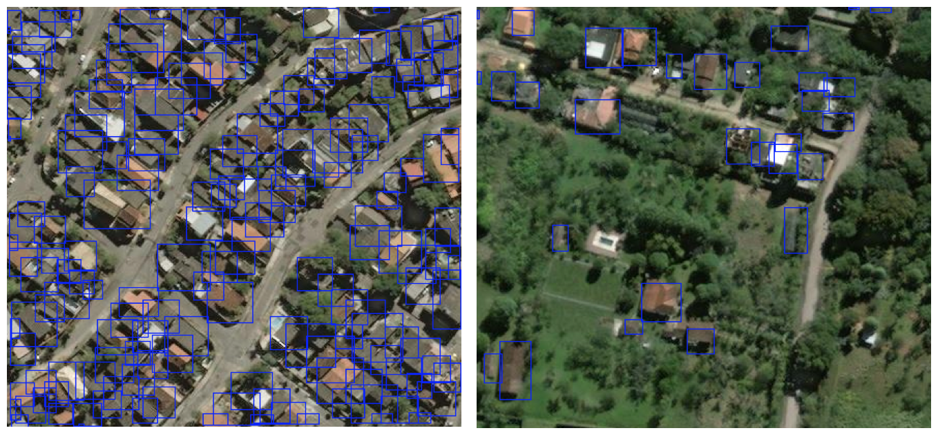
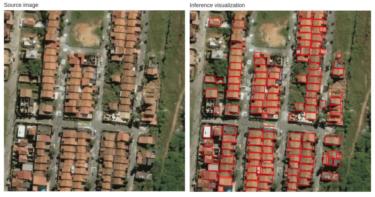
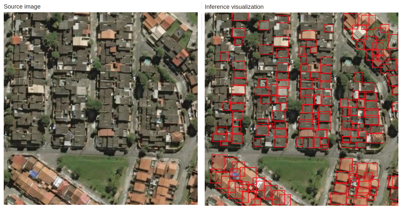
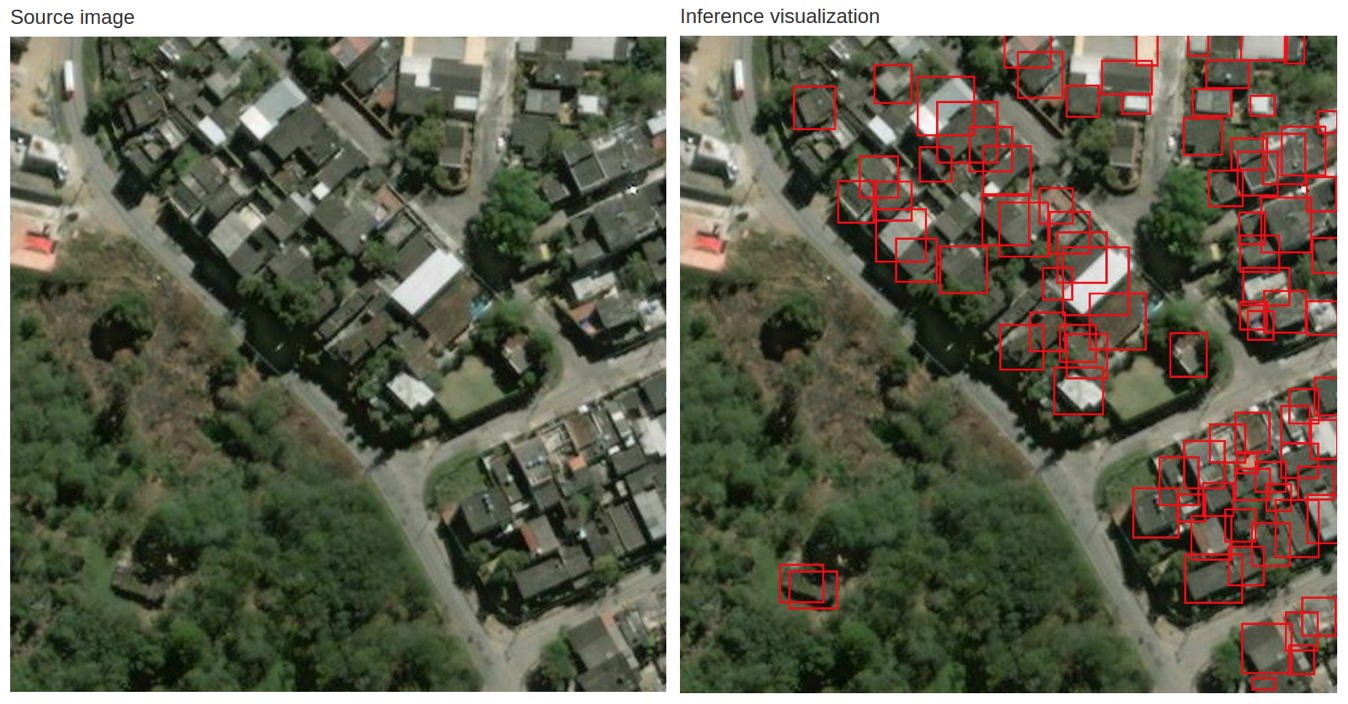
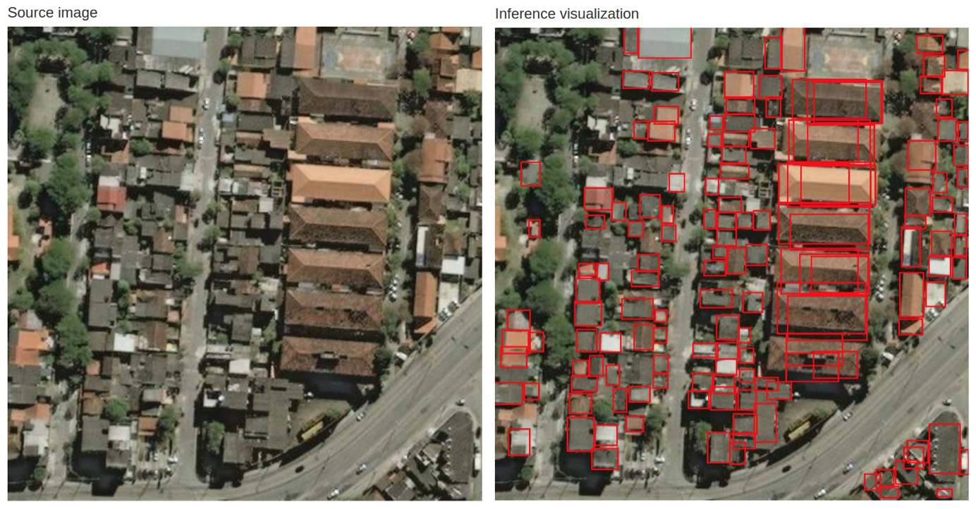
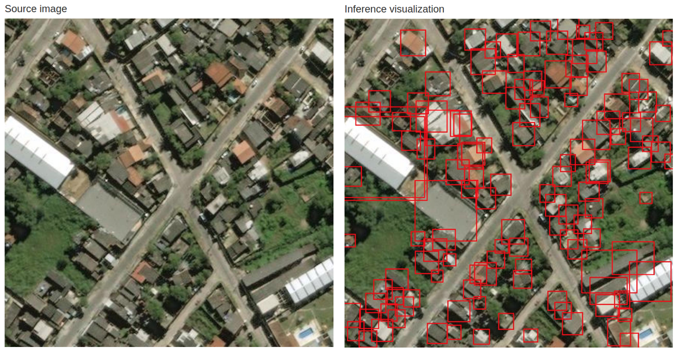
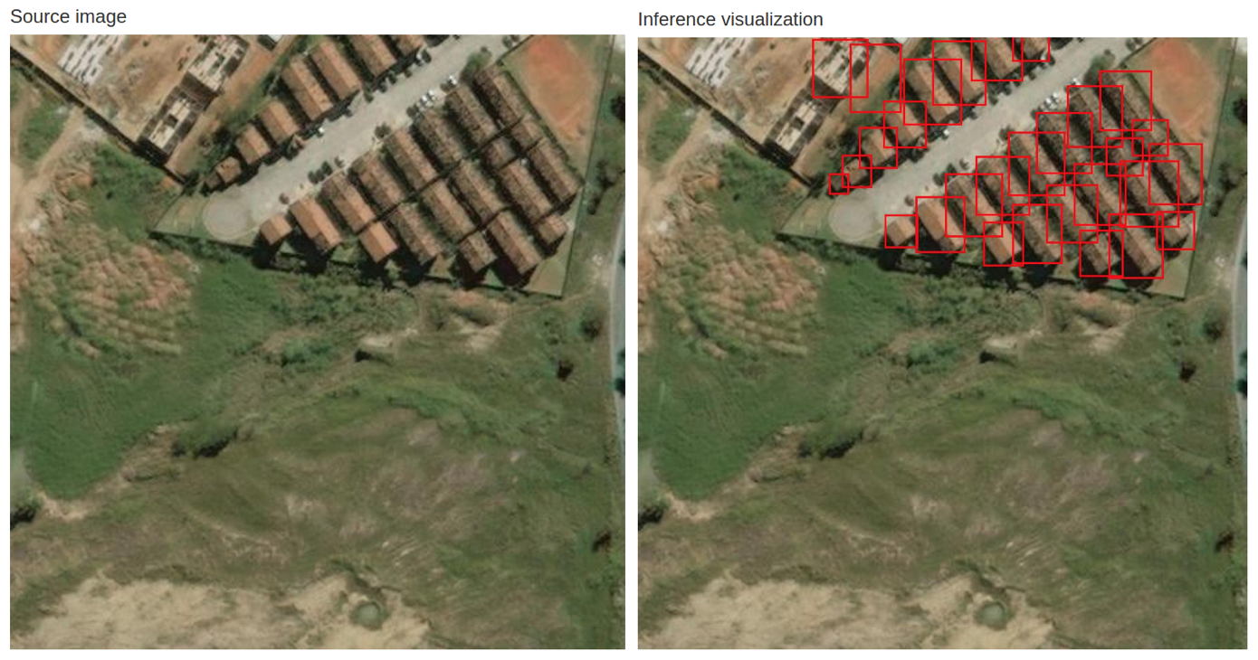
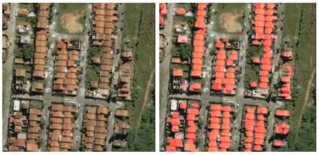
We followed the steps outlined in the DetectNet Parallel Forall post to train a modified version of DetectNet on the SpaceNet data. Training data for DetectNet consists of input images annotated with rectangular bounding boxes around objects to be detected. We resized all 3-band images to 1280 x 1280 pixels so that the majority of building bounding boxes would fall within the 50 x 50 to 400 x 400 pixel range in which DetectNet is sensitive. We then converted each building footprint to the smallest possible rectangle with sides parallel to the image that contains the original building footprint; this is the format required by DetectNet. We used a training dataset of 3552 images (filtered to only include images where no more than 50% of the image was blank/cropped pixels) and a randomly selected validation set of 259 images. Figure 3 shows two example training images with building bounding boxes as blue annotations.
Our initial attempts at training this modified version of DetectNet are promising; Figure 4 shows a selection of example validation images (left) and DetectNet’s predicted bounding boxes (right).
We modified the default DetectNet network by changing both network architecture and training parameters to achieve good convergence of both the training and validation loss. In particular, we changed the network input image dimensions to 1280 x 1280 and applied random cropping to 512 x 512 pixels at training time as a form of data augmentation. We changed the minimum allowable coverage map value for a bounding box candidate to be 0.06. We set the minimum allowable bounding box height to 10 pixels and the minimum number of bounding boxes that must be clustered to produce a final output bounding box to 4.
We trained the model with a batch size of 2 using the ADAM optimization algorithm with a learning rate of 1e-04 and an exponential learning rate decay. With these settings the trained network began detecting buildings after just one epoch and we trained for a total of 200 epochs.
We assessed DetectNet performance using the precision and recall metrics. The mean precision and recall values across the building bounding boxes in the validation set are 47% and 42% respectively.
We calculated these metrics by looping over all ground-truth bounding boxes in the validation dataset. For each ground-truth bounding box we looped over all predicted bounding boxes. If there exists a predicted bounding box whose Intersection Over Union (IOU) with the ground-truth bounding box is greater than 0.5 the prediction is considered a true positive. If a predicted bounding box does not have IOU greater than 0.5 with any ground-truth bounding box then it is a false positive. Fig 5 shows how IOU is calculated for a ground truth and predicted bounding box pair.
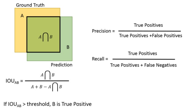
Precision is the number true positives divided by the total number of predicted bounding boxes, i.e. the percentage of relevant results. Recall, sometimes referred to as the sensitivity, is the number of true positives divided by the total number of ground truth bounding boxes. For both metrics higher is better.
These results confirm that it is possible to detect buildings and estimate bounding boxes using an object detection network even though there are a number of very small buildings relative to the image size with close proximity to one another. The limitation of this approach is that we are restricted to predicting bounding boxes whose sides are parallel to the input image and this certainly affects the precision of predicted bounding boxes. Furthermore, overlapping bounding boxes reduce recall. Therefore we evaluated a second approach that can account for varied building footprints and orientations to determine whether we can predict building footprints with higher accuracy. There is room for improvement in the object detection approach to building detection and we will cover some possible improvements in a forthcoming step-by-step tutorial on applying DetectNet to SpaceNet.
Approach 2: Semantic Segmentation
Another approach to building detection is semantic segmentation, support for which is currently under development in DIGITS. Semantic segmentation attempts to partition an image into regions of pixels that can be given a common label, such as “building”, “forest”, “road’ or “water”. See Figure 6 for an example. One approach to this would be to first segment the image into unlabelled regions and then try to assign a classification to each region. Alternatively, we could attempt to independently classify each pixel in the image and then extract segments with a common pixel class that correspond to an individual object. We chose to use the second approach—sometimes called instanced segmentation—in this work.
![Figure 6: An example of semantic image segmentation [Everingham 2012].](https://developer.nvidia.com/blog/parallelforall/wp-content/uploads/2016/08/Figure6.png)
Training data for semantic segmentation has labels associated with each training image that are themselves an image with pixel values corresponding to the target class of the pixel. In formulating our segmentation dataset we followed work done at Oak Ridge National Laboratory [Yuan 2016]. This work demonstrated state-of-the-art results for pixel-wise semantic segmentation of 30 cm resolution aerial imagery for building footprint extraction. We used Yuan’s approach of computing the signed distance function for our objective classes rather than “building” or “not building”. After applying this function to the building footprint outlines each pixel value is equal to the distance to the closest point on a building outline. Pixels inside buildings have positive distance values and pixels outside have negative values. Figure 7 shows an example training image and the corresponding label image.
As described in [Yuan 2016], there are two advantages to this representation: 1) Boundaries and regions are captured in a single representation and can be easily read out (boundaries are zero and regions are positive values). 2) Training with this representation forces a network to learn more information about spatial layouts (e.g., the difference between locations near buildings and those far away).
We ingested all of the 3-band SpaceNet images that contained at least one building along with their labels in the signed distance format as grayscale images. We binned the signed distance function values into 128 bins ranging in value from 64 to 192. These values became the integer pixel value in the label image. All images and labels were resized to 512 x 512 pixels, and we reserved 5% of the data for model validation.
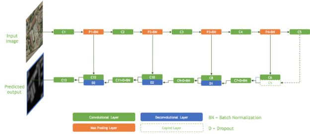
We trained a fully-convolutional neural network (FCN) for semantic segmentation with an architecture inspired by the recently published SharpMask from Facebook AI Research (FAIR) [Pinheiro et al. 2016]. Figure 8 shows our network architecture. It has become common in semantic segmentation applications to adopt the general structure of a FCN that first performs feature extraction on the image using stacked convolutional layers and then uses one or more deconvolutional layers to upsample these feature maps to the same size as the label image. In other words we attempt to directly predict the pixel values in the label image. FAIR showed how to refine the output from these network architectures to generate higher-fidelity masks that more accurately delineate object boundaries. A typical FCN for semantic segmentation predicts coarse segmentations in the feed forward pass. The SharpMask architecture then reverses the flow of information and refines the coarse predictions by using features from progressively earlier layers in the network. FAIR provided the following intuitive explanation in their excellent blog post: to capture general object shape, you have to have a high-level understanding of what you are looking at provided by the FCN, but to accurately place the boundaries you need to look back at lower-level features all the way down to the pixels (SharpMask). In essence, we aim to make use of information from all layers of a network, with minimal additional overhead.
We also note that Noh et al. [2015] demonstrated the improvement in segmentation of detailed shapes gained by learning the deconvolutional filters used in upsampling layers rather than using just fixed bilinear filters as had been common in earlier segmentation networks. As such, we made the filters of our final deconvolutional layer trainable. Noh et al. also noted the importance of batch normalization, which we also incorporated at various layers.
The objective function for the network is the average Euclidean distance between the true and predicted pixel values.
For training and validation we restricted the dataset to 3-band SpaceNet images containing at least one building footprint. Our dataset consisted of 4174 and 220 images for training and validation, respectively; we used only images with at least one non-zero pixel. We trained the model with a batch size of 17 using the ADAM optimizer and exponential learning rate decay for 100 epochs. Training took approximately 3.5 hours on an NVIDIA Titan X (Pascal) GPU using NVIDIA Caffe 0.15.8 and cuDNN 5.1.
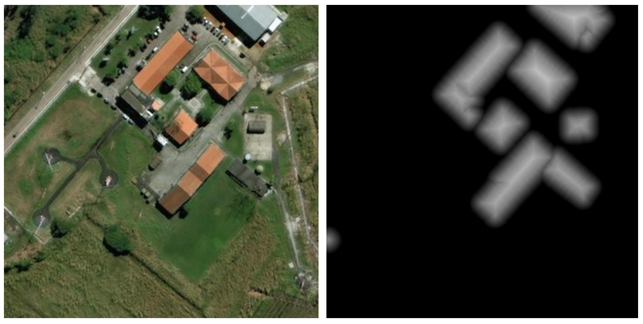
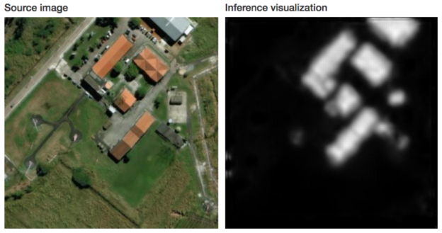
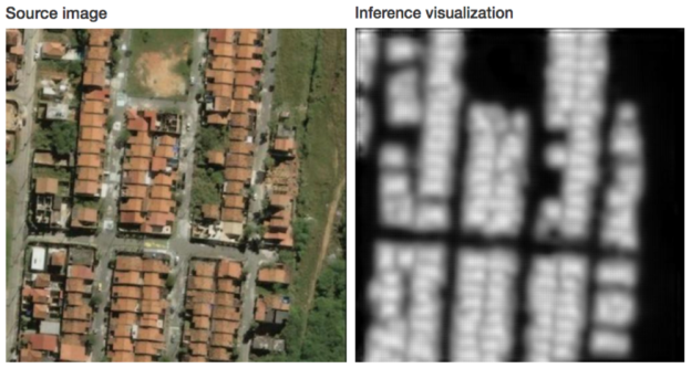
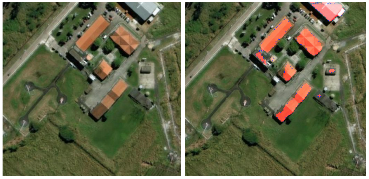
By the end of training the network was able to clearly identify regions in input images containing buildings and in many cases the signed distance image had sufficient accuracy to segment individual buildings. Figure 9 shows two example validation images and the corresponding predicted signed distance image outputs as visualized by DIGITS.
In order to obtain a final segmentation of the image into building versus not-building regions we apply a simple thresholding around the pixel value 128. Recall that in the training labels pixels with the value 128 fall on the outline of buildings. Therefore we label pixels with values greater than 128 as building pixels. Figure 10 shows a selection of validation images and the thresholded signed distance output overlaid on the image. 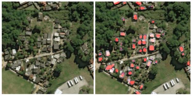
The mean per-pixel Euclidean distance between the ground truth signed distance image and the predicted signed distance image is 1.33 for the validation dataset. This makes the segmentation method an effective solution for general land usage classification into the classes building and not-building. In the case of images with large, well separated buildings we can see that the thresholding method can effectively segment individual buildings and these segments could be used to provide more accurate building footprints for buildings with complex shapes. However, when there are many small buildings close together the current thresholding method often fails to effectively separate individual buildings.
Getting started with DIGITS and SpaceNet
We have demonstrated two methods for detecting buildings in the SpaceNet 3-band data. In a future post we will give step-by-step instruction for replicating these results and describe improvements that can be made to the data preprocessing, model and training process to further improve the accuracy of the outlines of individual building footprints.
In the meantime, you can download the SpaceNet data here. DIGITS 4 has all the functionality to replicate the object detection approach to building detection. Go to developer.nvidia.com/digits to get started. The developmental functionality required to implement a semantic segmentation approach to building detection is available in the open-source DIGITS github project. You can download the prototxt files for both the DetectNet and segmentation network architectures described in this post here. We look forward to your feedback and contributions on Github as we continue to develop it.
References
[Yuan 2016] Jiangye Yuan, Automatic Building Extraction in Aerial Scenes Using Convolutional Networks, arXiv:1602.06564, 2016
[Pinheiro et al. 2016] SharpMask: Learning to Refine Object Segments. Pedro O. Pinheiro, Tsung-Yi Lin, Ronan Collobert, Piotr Dollàr (ECCV 2016)
[Ren et al. 2015] Shaoqing Ren, Kaiming He, Ross Girshick, Jian Sun, Faster R-CNN: Towards Real-Time Object Detection with Region Proposal Networks, arXiv:1506.01497, 2015
[Redmon et al. 2015] Joseph Redmon, Santosh Divvala, Ross Girshick, Ali Farhadi, You Only Look Once: Unified, Real-Time Object Detection, arXiv:1506.02640, 2015
[DigitalGlobe 2014] DigitalGlobe Core Imagery Product Guide v. 2.0.
[Everingham 2012] Everingham, M. and Van-Gool, L. and Williams, C. K. I. and Winn, J. and Zisserman, A., The PASCAL Visual Object Classes Challenge 2012 (VOC2012) Results
[Gonzalez 2008] Rafael Gonzalez and Richard Woods. (2008) Digital Image Processing. New Jersey: Pearson Prentice Hall