Cluster Analysis
Cluster Analysis is the grouping of objects based on their characteristics such that there is high intra‐cluster similarity and low inter‐cluster similarity. The classification into clusters is done using criterion such as smallest distances, density of data points, or various statistical distributions. Cluster analysis is a Graph Analytics application and has wide applicability including in machine learning, data mining, statistics, image processing and numerous physical and social science applications.
In many applications we can describe the data set as a graph  , where vertices
  represent items and edges
  represent relationships between them. It is often desired to
split the graph into separate sub‐graphs that represent different groups or clusters, such as communities in social
networks. The optimal solution is often infeasible to compute since the problem is NP‐hard; in practice it is better
to use a smart approximation method in order to get a result in reasonable time. There are many ways
of determining these groups. For example, we can find the clusters based on the minimum balanced cut,
modularity, flow, and betweenness centrality metrics.
represent relationships between them. It is often desired to
split the graph into separate sub‐graphs that represent different groups or clusters, such as communities in social
networks. The optimal solution is often infeasible to compute since the problem is NP‐hard; in practice it is better
to use a smart approximation method in order to get a result in reasonable time. There are many ways
of determining these groups. For example, we can find the clusters based on the minimum balanced cut,
modularity, flow, and betweenness centrality metrics.
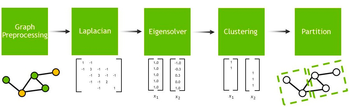
Spectral Clustering
The spectral clustering scheme constructs the graph Laplacian matrix, solves an associated eigenvalue problem, and extracts splitting information from the calculated eigenvector(s).
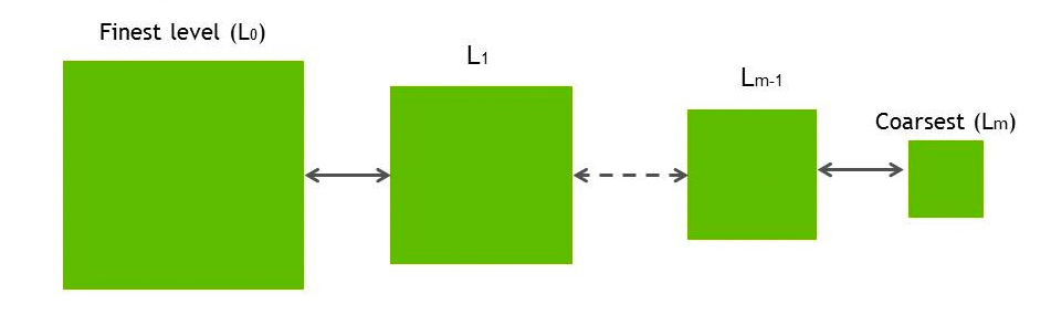
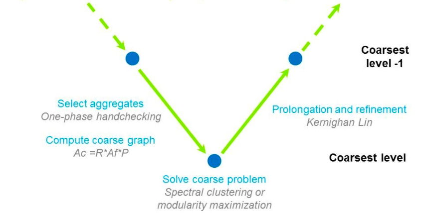
Hierarchical Clustering
The hierachical clustering scheme constructs a hierarchy of related graphs starting from a finest level (original) and proceeding to a coarsest level. Each level of the hierarchy is constructed from the previous level by collapsing nodes and edges together based on a set of heuristics. For example, contracting a single edge called ‘heaviest’ in some metric, which removes a single vertex and edge, or replacing groups of vertices with a single ‘representative’ vertex and removing all edges ‘interior’ to the group at once. In a way this is similar to the techniques often used in algebraic multigrid, implemented in the AmgX library. This multi‐level scheme can be a clustering technique by itself or it can also be combined with other approaches. The clustering problem is then solved on the coarsest level, potentially using spectral clustering, and the results propagated back to the fine level, usually with some Kernighan‐Lin ‘smoothing’ along partition boundaries as each finer level is partitioned by reversing the contraction done previously to cast the coarsest level partition upward through the hierarchy. This approach is nearly optimal for low‐degree graphs or graphs with a regular structure such as finite element or finite volume connectivity graphs or graphs arising from PDE discretizations in general.
Clustering Metrics:
Minimum balanced cut metric measures the size of each cluster and the number of connections between clusters. It attempts to preserve the same size for each cluster, while minimizing the number of connections between them. It can be computed using spectral and/or hierarchical clustering approaches, also called multi‐level schemes.
Modularity metric measures the density of connections within a cluster compared to the total number of edges in the graph. The technique is related to spectral partitioning in the sense that it also solves an eigenvalue problem with an auxiliary matrix and extracts the splitting from it. However, the auxiliary matrix is constructed differently: using Bij =Aij – kikj/2m, where A is the adjacency matrix, m is the total number of edges in the graph and ki, kj are the number of neighbors of vertex i and j, respectively. This is often a ‘natural’ metric for biologically related graphs, such as gene interactions or evolutionary graphs of related species, and works well for community detection. We can also split the graph into two parts by cutting a carefully selected set of edges, so as to maximize the modularity metric of the clusters created. This metric can often be useful in transportation and routing networks as a measure of their connectivity, or to discover tightly connected social ‘cliques’ from social networks.
Flow metric measures the flow capacity achieved on each edge and can be used to split the graph on the edge(s) that contain the maximum/minimum flow. In a way it is similar to the betweenness centrality metric which measures the number of shortest paths going through a particular vertex and can be used to split the graph into clusters based on such a vertex. Applications of the flow metric include detecting weak points in a computer network, planning power grid expansion, and identifying connecting bridges between communities.
Clustering vs Partitioning:
It is important to outline the difference between the clustering and partitioning approaches. The differences are subtle, but important. Clustering is often used in analysis of graphs and networks, while partitioning is often used in HPC for load balancing across a fixed set of resources. For example, in partitioning the size and often the number of sub‐graphs is specified and fixed, while in clustering the number is unknown and an output from rather than an input to the process. Partitioning forces you to find a solution, while in clustering the lack of clusters might be a result in itself that tells you something about the data.
Notice that the relationship between partitioning and clustering is particularly interesting for the
minimum balanced cut metric. This metric attempts to keep the size of the sub‐graphs the same, but it
does not have a hard limit, such as the size of a cluster being within a threshold  of an average
 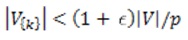 , where V is the set of vertices for the whole graph,
  is the set of
vertices assigned to partition k, p is the number of partitions and |.| is the cardinality of a set. A hard
limit can be imposed during the extraction of sub‐graphs, either in the k‐means algorithm or during the
local refinement using methods such as Kernighan‐Lin and Fiduccia‐Mattheyses. It is important to keep
this point in mind when using these clustering schemes.
is the set of
vertices assigned to partition k, p is the number of partitions and |.| is the cardinality of a set. A hard
limit can be imposed during the extraction of sub‐graphs, either in the k‐means algorithm or during the
local refinement using methods such as Kernighan‐Lin and Fiduccia‐Mattheyses. It is important to keep
this point in mind when using these clustering schemes.
Accelerating Cluster Analysis with GPUs
Cluster analysis is a problem with significant parallelism and can be accelerated by using GPUs. The NVIDIA Graph Analytics library (nvGRAPH) will provide both spectral and hierarchical clustering/partitioning techniques based on the minimum balanced cut metric in the future. The nvGRAPH library is freely available as part of the CUDA Toolkit. For more information about graphs, please refer to the Graph Analytics page.
Additional Resources:
1. "Fast Spectral Graph Partitioning on GPUs." Naumov, Maxim. Parallel For All. NVIDIA, 12 May 2016.
2. "GPU‐Accelerated R in the Cloud with Teraproc Cluster‐as‐a‐Service.", Sissons, Gord. Parallel ForAll. NVIDIA, 02 June 2015.
3. "Parallel Spectral Graph Partitioning" Naumov, Maxim (NVIDIA) and Moon,Timothy March 2016