 It’s that time again — SpaceNet raised the bar in their third challenge to detect road-networks in overhead imagery around the world. Today, map features such as roads, building footprints, and points of interest are primarily created through manual techniques. In the third SpaceNet challenge, competitors were tasked with finding automated methods for extracting map-ready road networks from high-resolution satellite imagery. This move towards automated extraction of road networks will help bring innovation to computer vision methodologies applied to high-resolution satellite imagery and ultimately help create better maps where they are needed most such as humanitarian efforts, disaster response, and operations. For more details, check out the SpaceNet data repository on AWS and see our previous NVIDIA Developer Blog post on past SpaceNet challenges to extract building footprints.
In this post, we approach the current SpaceNet challenge from distinct perspectives. The first part of this blog describes how to directly leverage the full 8-band imagery and manipulate ground truth labels to obtain excellent road networks with relative ease and excellent performance. We next look at how we might exploit the material properties of the road surface itself by using the spectral aspect of the data to create a deep learning solution tailored for a specific spectral signature. Finally, we take creative liberties to think about how we might apply these types of deep learning solutions in a broader operational sense using conditional random fields, percolation theory, and reinforcement learning. Think of this like Bohemian Rhapsody for deep learning (minus the Grammy Hall of Fame).
Section 1 – Tiramisu and Manipulating the Truth
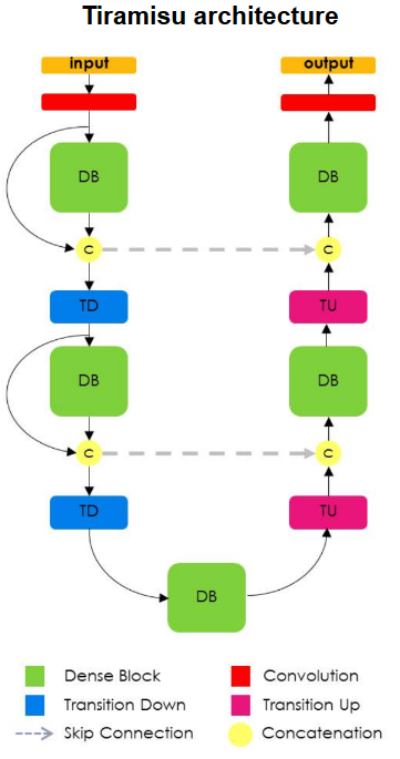
In this section the Tiramisu network is used which is readily available in many forms on GitHub. Here we use the Semantic Segmentation Suite, written by George Seif, which incorporates many different segmentation methods. This network was chosen because it can provide highly accurate semantic segmentation masks for a variety of segmentation tasks and easily extends to the full 8-channel data (in contrast to just 3-channel RGB data). From a design perspective, Tiramisu extends the U-Net architecture adding Densely Connected Convolutional Networks into the network through conversion into fully convolutional layers to enable upsampling. The advantages of these modifications include deeper supervision between layers. Given that the feature maps are shared throughout the dense blocks this aids multi-scale supervision and introduces skip connections within and outside of each block, a feature shown to be extremely successful in Residual Networks.
To infer road networks using the SpaceNet data a number of preprocessing steps are required to create segmentation masks for training and evaluation. The tool sets provided by Cosmiq Works provide useful methods to convert from the line string graph formats into a segmentation mask allowing the user to specify the width of the segmented road. It is possible to generate a segmentation model with these tools, however it is evident upon visual inspection that these segmentation masks do not label all pixels which are associated with roads, highways and alleyways. For example a segment may either be too wide or too narrow to describe a specific road. In the case of a label being too wide this results in buildings, trees and other objects to be labelled incorrectly as road. Conversely, a too narrow label will result in potentially large areas of the road network being labelled as the background class. In some cases areas which clearly contain roads are not labelled as such. This label mixing can adversely affect accuracy, particularly at large intersections which, as described in the Cosmiq Works blog, are extremely important to label correctly to maximize the Average Path Length Similarity (APLS) metric.
Label Pre-Processing
To reduce this label misassignment we can use relatively straightforward image processing approaches. Whilst these approaches will not completely rectify the problem they will increase the number of pixels correctly labelled as a drivable surface and background classes. To achieve this the OpenCV floodFill function is employed. From the OpenCV website:
The functions floodFill fill a connected component starting from the seed point with the specified color. The connectivity is determined by the color/brightness closeness of the neighbor pixels. The pixel at (x,y) is considered to belong to the repainted domain if:
![]()
![]()
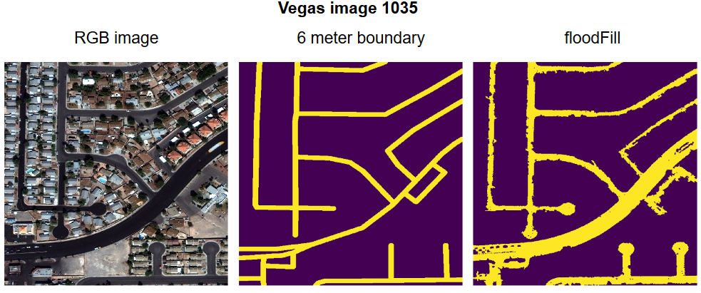
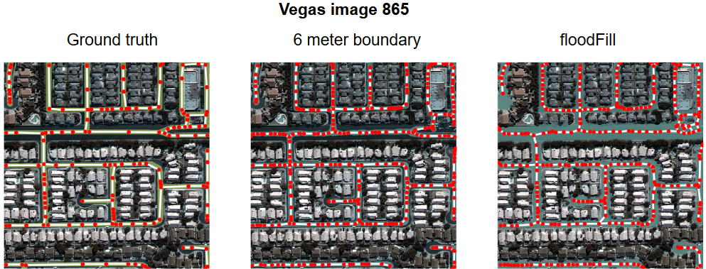
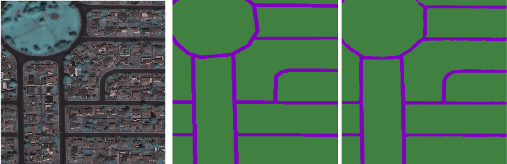
The floodFill function effectively generates a mask for all connected points which fulfil the above statement. Using this method it is possible to use a thinned version of the segmentation mask created by the Cosmiq Works functions to specify seed points for the floodFill function. Examples of the Las Vegas dataset processed using the Cosmiq Works and the floodFill methods are presented below in figure 2 (left: image, middle: Cosmiq Works boundary method, right: floodFill segmentation). It is clear that many more pixels are correctly labelled, particularly in parking lots, cul-de-sacs, and major trunk roads. In addition objects on or overhanging roads such as vehicles and vegetation are no longer labelled incorrectly.
The Tiramisu network is trained using Tensorflow on the full 8 band Vegas AOI dataset. The Cosmiq Works mask tool and the floodFill method are used for label generation and model accuracy is calculated using mean Intersection over Union (IoU) for both road and background classes and using the APLS metric. In all cases the networks were trained for 14 epochs taking approximately 6 hours per model per dataset per GPU when using NVIDIA Quadro GP100 GPUs. When using 8 band data the number of initial convolutional filters in the Tiramisu network is increased from 64 to 96 to increase the network capacity to learn multispectral features. The proportion of training, validation and test data is 70%, 15% and 15% respectively.
Results
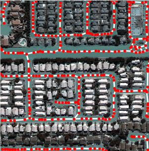
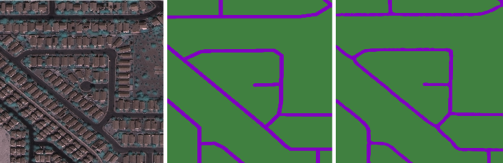
Figure 3 shows the resulting masks from this process using the Tiramisu network on hold out test data. The left image presents the ground truth mask and graph, middle predicted mask and graph using the Cosmiq Work’s boundary function, and the right image shows predicted mask and graph using the floodFill approach. The floodFill is clearly superior when compared to the boundary fill method. The wide highway and it’s junctions are detected which is advantageous when calculating APLS. However care must be taken in areas where floodFill selects areas which are clearly drivable, such as parking lots and side roads, which are not labelled in the ground truth images.
The Tiramisu network trained on all 8 bands achieved a very respectable mean IoU of 0.89 and mean APLS of 0.60. This was achieved through simple image preprocessing and postprocessing steps and by training a standard open source model against the full dimensionality of the dataset without any major changes or additions.
Wrapping Up
In this section we have discussed some image processing methods to aid data preparation which can significantly increase accuracy in some cases. Data labelling and formatting is at the heart of data science and artificial intelligence. Depending on the overall goals of your requirements the correct selection of data preprocessing methods, and selecting the most relevant set of evaluation metrics, can help you achieve them.
In the next section we focus on determining the best spectral content to use when training a deep learning network for a specific spectral signature.
Section 2: Focusing the Spectrum
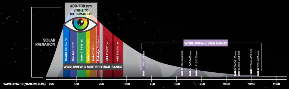
In this section we want to think about the physical properties of the road materials we are trying to isolate as well as the surrounding observable environment and how the sensor’s characteristics might be able to help in the road extraction task. That is, we want to exploit material-specific spectral signatures within the imagery for efficient asset detection and localization. The SpaceNet road challenge data were collected by the DigitalGlobe Worldview-3 satellite. The 8-band multispectral images contain spectral bands for coastal blue, blue, green, yellow, red, red edge, near infrared 1 (NIR1) and near infrared 2 (NIR2) (with corresponding center wavelengths of 427, 478, 546, 608, 659, 724, 833 and 949 nm, respectively). This extended spectral range allows Worldview-3 imagery to be used to classify the actual material that is being imaged as shown in Figure 4 .
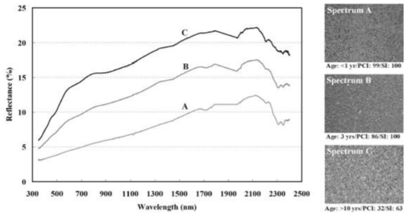
Spectral features for a given material can be thought of physical characteristics of the material that manifest as observed reflectance (or absorbance) changes at particular wavelengths. Traditional spectral analysis leverages these diagnostic features to perform material identification. For example, organic materials such as vegetation exhibit very distinct spectral features in the red and near-infrared (NIR) portion of the spectrum. These features are driven largely by the chlorophyll content of vegetation. Chlorophyll will strongly absorb energy in the visible portion of the spectrum and strongly reflect energy beginning in the red/near-infrared (wavelengths ~700 nm and longer).
Given that we are interested in roads, why do we care about vegetation? As you can see from Figure 5, asphalt tends to be a poor reflector in the red and near-infrared portions of the spectrum. In fact, man-made objects in general will exhibit this poor reflectance characteristic. These differences will manifest as a strong contrast between vegetation and manmade objects in the last three spectral bands of the Worldview 3 sensor which is easily exploited with deep learning.
Of course, this is not an exhaustive spectral analysis of all environments observed in the SpaceNet data but it does motivate the investigation of a pure R/NIR deep learning model. The additional caveat here is that this data has not been compensated for atmospheric effects and that has the potential to affect results. For the sake of simplicity, we will assume that the atmospheric properties are constant over the entire Las Vegas AOI. That is, the atmosphere distorts all AOI-2 images in the same way. And, since Las Vegas is a dry desert-like climate, it is reasonable to assume minimal atmospheric distortion.
Something else to keep in mind is that the bit depth of the imagery from satellite sensors is often higher than 8-bit. However, the majority of deep learning frameworks and generic image manipulation libraries cannot handle data with higher bit depths. In combination with tools such as numpy, one can convert the data down to the required 8-bit depth and use it in subsequent steps. The sample code below provides two methods for extracting band information and using numpy and scipy’s bytescale function to perform a contrast stretch on the raw data that clips the top 10% and bottom 2% of values.
def retrieve_bands(ds, x_size, y_size, bands):

    stack = np.zeros([x_size, y_size, len(bands)])

    for i, band in enumerate(bands):
        src_band = ds.GetRasterBand(band)
        band_arr = src_band.ReadAsArray()
        stack[:, :, i] = band_arr

    return stack


def contrast_stretch(np_img, p1_clip=2, p2_clip=90):

    x, y, bands = np_img.shape
    return_stack = np.zeros([x, y, bands], dtype=np.uint8)
    for b in range(bands):
        cur_b = np_img[:, :, b]
        p1_pix, p2_pix = np.percentile(cur_b, (p1_clip, p2_clip))
        return_stack[:, :, b] = bytescale(exposure.rescale_intensity(cur_b, out_range=(p1_pix, p2_pix)))

    return return_stack
Segmenting road networks from R/NIR data
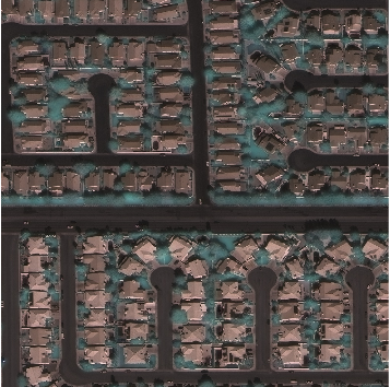
The last 3 bands of the MSI pan-sharpened imagery were extracted from the original imagery for AOI-2 in Las Vegas (i.e. red edge, NIR1, and NIR2). Each image was resized to 1024×1024 and scaled to 8-bits with a contrast stretch clips of 2% and 90%. Ground truth masks did not make use of any additional pre-processing (i.e. flood fill). Training and validation datasets were created with a typical 20% split. A sample R/NIR training image is show below. It is interesting to note the pan-sharpening artifacts manifesting as blur in the vegetation, namely trees.
The same Tiramisu architecture (described in section 1) was used again for this exercise. Since we are using a fully convolutional network (FCN) we are not restricted by input size at inference, however it does need to be a multiple of the original training dimensions. For this effort a training size of 512×512 was chosen. Conveniently, Geospatial Data Abstraction Library (GDAL) includes method calls to resize geospatial datasets while preserving the geographic metadata via a warping function. For added functionality, this can either be done in a file or in memory, depending on where you chose to insert this process in your workflow. The sample code below shows the GDAL API call used to do a resize in memory.
warp_ds = gdal.Warp('', img_fn, format='MEM', width=resize[0],
height=resize[1],

resampleAlg=gdal.GRIORA_NearestNeighbour, outputType=gdal.GDT_Byte)
Results
The model was trained for ~50 epochs with a batch size of 1 on the R/NIR data for Vegas. Shown below are some samples from the segmentation results generated by the model.
The segmentation results were processed using some custom tools and the provided APIs and tools to extract a road network (represented by a graph) and calculate the APLS score per image. Below are the companion road network predictions for the presented samples.
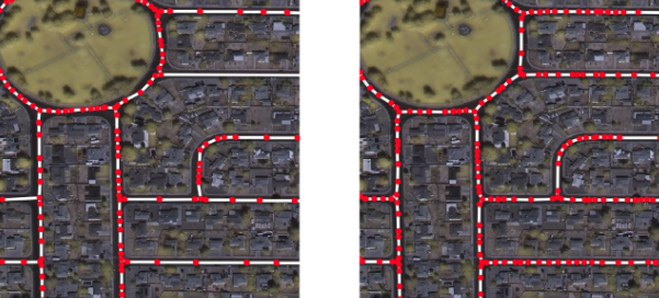
The model trained on only the R/NIR data produced a mean IoU of 0.71 and a mean APLS score of 0.56
Wrapping Up
Above we discussed using a subset of the spectral data to train a deep learning model for road extraction. While there are a few implicit assumptions in this approach (e.g. atmospheric corrections), this method significantly reduces the amount of data needed for model training by focusing on a specific spectral signature. Compared to the full 8-band model, these R/NIR model results are slightly degraded but potentially more desirable given the data reduction and elimination of pre-processing overhead (i.e. flood-fill). Although, the minor performance reduction could simply be due to the fact that this approach uses a lot less data!
In the next section we are going to go off the beaten path and think about things slightly differently.
Section 3: Thinking Outside the Box
In this section we leverage the NVIDIA GPU Cloud resources together with the next-generation of AWS EC2 compute-optimized GPU instances. The AWS P3 instances are powered by up to 8 of the latest-generation NVIDIA Tesla V100 GPUs and are ideal for computationally advanced workloads such as machine learning (ML), high performance computing (HPC), data compression, and cryptography. Based on NVIDIA’s latest Volta architecture, each Tesla V100 GPU provides up to 125 TOPS of mixed-precision performance, 15.7 TFLOPS of single precision (FP32) performance and 7.8 TFLOPS of double precision (FP64) performance. For machine learning and deep learning applications, the P3 instance offers up to 14x performance improvement over previous P2 instances based on the much older NVIDIA Tesla K80 GPUs, allowing developers to train their machine learning models in hours rather than days.
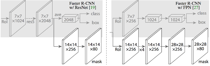
For road segmentation we utilize the awesome Mask R-CNN deep learning network architecture implemented by Matterport available on GitHub. Mask R-CNN is a flexible framework for object instance segmentation which efficiently detects objects in an image while concurrently generating high-quality segmentation masks for each instance. To do this, Mask R-CNN extends Faster R-CNN by adding an additional branch for predicting an object mask together with the original branch for bounding boxes.
For training Mask R-CNN we start with the model sufficiently trained in advance on MS COCO data. The network is configured with 128 training ROIs per image, RPN anchor scales of (8, 16, 32, 64, 128), and an RGB pan-sharpened input image size of 512x512x3. Over all four areas of interest in the SpaceNet dataset there are 2731 total training images with associated ground truth road labels. These data were divided into a 90/10 split of 2458 images used to further train the network and 273 holdout images for validation. A training image label consists of an arbitrary number of road lines each specified as list of points in pixel space. Bresenham’s line algorithm was used convert these lines to binary segmentation mask labels for network training. It is important to note that Mask R-CNN is an object detection network at heart and therefore each road line must be treated as a separate object mask rather than combining all road lines into a single binary mask of size 512×512. That is, if a training image specified N road lines then the associated training label for that image would be a binary mask of size 512x512xN where label[:,:,i] is the binary mask for the i’th road line. The network used here was trained with a batch size of 8 images for 40 total epoch with 300 steps per epoch.
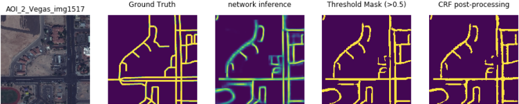
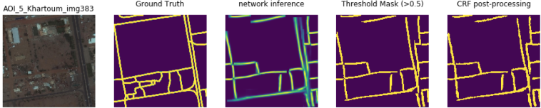
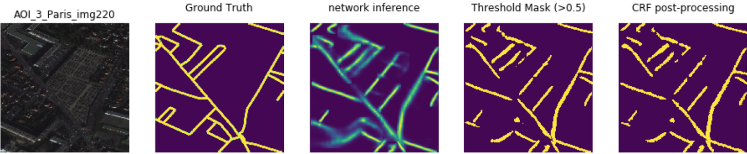
A traditional approach for working with object detectors is to threshold detections scores (confidence metric from 0 to 1) at 0.5 so that detections scoring less than 0.5 are discarded. Similarly, the segmentation mask produced by the Mask R-CNN network provides a softmax probability for each image pixel as “road” or “not-road”. Those pixels scoring, say, 0.87 have high probability of being road while a pixel score of 0.21 would be a weak indication of “road”. Therefore, a common post-processing approach is to binarize the resulting segmentation mask by converting all softmax probabilities below 0.5 to 0 and all probabilities 0.5 and above to 1.
Another popular approach to aid in the pixel classification decision processes is a technique called conditional random fields (CRFs) which is often employed for “structured prediction” in pattern recognition and hence readily applied in semantic segmentation post-processing. Essentially, a CRF is a probabilistic graphical model that encodes known relationships between observations and produces interpretations consistent with those relationships. A discrete classifier such as threshold classifier described above, on the other hand, predicts a label for a single sample without considering “neighboring” samples while a CRF can take context into account. It is crucially important to view the deep learning network as a technique for producing information that informs a decision process rather than a device that makes a decision.
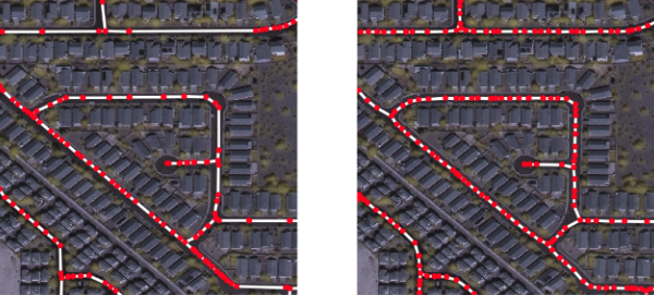
Here are a few Mask R-CNN results with the aforementioned post-processing approaches:
Applications
In this section we want to highlight how we might work with and apply this data for real operations. At this point, given some overhead image we can produce an “educated” guess for where roads might be within that image. So, now what? For starters, given a map of interconnected roads we can start to ask basic questions like “can we get from A to B?” or similarly “what are all the traversable locations from location X?” Just because two points are “connected” does not inform us for exactly how we might actually go about getting from point A to B. Notice that creating a simple binary test (yes/no) for
bool = is_connected(mask,A,B)
is quite computationally efficient compared to something like “find the optimal path from A to B”. This raises another question, given some road segmentation mask, what is meant by “optimal path” between two points? In routing applications we often think of “optimal” as “shortest” and/or “fastest” but here we also have to consider that we’re not entirely certain where the road actually is. We can therefore start to think about things like the maximum likelihood route between two points (hint: it is not likely going to be the shortest route). Again, this underpins the notion that the deep learning network as a technique for producing information that informs a decision process.
Percolation
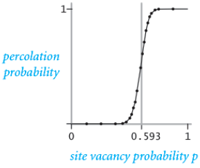
If we think of an image as a grid of vertices with edges between vertices (i.e. pixels) with probability p, the description is strikingly similar to a domain of statistical physics called percolation theory. In general, percolation refers to the movement of fluids through porous materials and over the last decades the theory of percolation has brought new understanding and techniques to a broad range of topics in physics, materials science, complex networks, epidemiology, and other fields. A famous problem in percolation theory involves systems comprised of randomly distributed insulating and metallic materials: what fraction of the materials need to be metallic so that the composite system is an electrical conductor? If a current passes through the system from top to bottom then the system is said to percolate. In such a system a site (i.e. grid point) is “open” or “vacant” with probability p and “blocked” with probability q = (1-p).
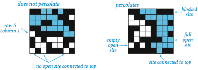
What makes this problem famous is the system phase change that occurs above a critical vacancy probability Pc. That is, systems with site vacancy below the critical threshold, p < Pc, almost never percolate and systems with p > Pc almost always percolate.
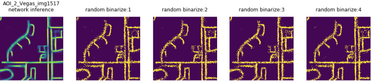
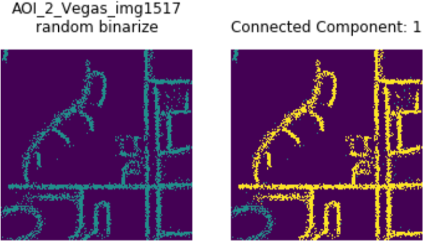
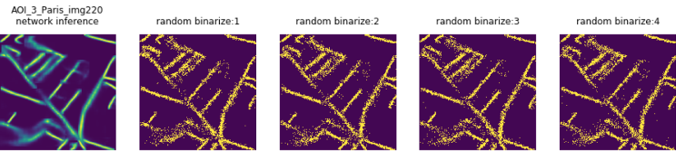
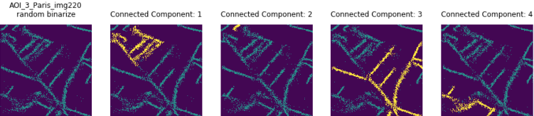
Since the segmentation mask provides a probability for each pixel we can think of each pixel as a Bernoulli random variable. That is, think of each pixel as a biased coin that when flipped produces heads with probability p and talis with the “leftover” probability of q = (1-p) — just like the site percolation problem above. In this way we create a binary (0 or 1) mask where each pixel is assigned heads = “road” = 1 or tails = “not-road” = 0. Once we have a random road network realization we can grow (i.e. percolate) connected components. Below shows a few examples of using the segmentation softmax probabilities to produce random realization of the road network and their associated connected components. For any two points in a connected component, there exists a path between those points.
Routing versus Navigation
Percolation was a useful way to investigate connected components and build a deeper understanding for connectivity from a probabilistic perspective which provided a simple yet robust formalism for testing if two points were connected. However, from an operations standpoint, given some objective or goal we really need to use the information provided for routing purposes. That is, how do we move beyond probabilistic connectivity to more useful capabilities such as optimal navigation of the environment? Given some graph of vertices and edges we can, no doubt, compute the shortest path between points. Although, if we consider an image with dimensions 512×512 pixels that translates to a graph with 266,144 vertices which means shortest path computations will scale poorly as the environment size increases. For example, Dijkstra’s algorithm has worst case performance of O(|E| + |V|log(|V|)) where |E| is the number of edges and |V| is the number of vertices and for grid graph of size {h,w} we have |V| = nm and |E| has a maximum possible value of (n-1)m + (m-1)n. With the native image resolution of 1300×1300, the SpaceNet roads challenge data produces graphs with 1,690,000 vertices and 3,377,400 possible edges. These numbers quickly become intractable for 4k and 8k overhead imagery. Operationally, given some goal location, it can be quite computationally expensive to determine shortest path from an arbitrary location on-the-fly. Furthermore, we still need to incorporate the environmental uncertainty of where the road actually is! Another option to consider is the A algorithm (pronounce “A star”) which generally achieves better performance by using heuristics (i.e. environmental informance in this case) to guide the search process. The A* algorithm is an informed best-first search process where the search considers the vertices that appear to lead most quickly to the goal. While A* can incorporate environmental information to the search process and thus typically converge faster to a path between two points, there are still some things to think about. For example, these routing approaches work well if we know exactly the starting point to the goal. However, if for some reason we find ourselves in a totally different location on the map we then need a new route computed to the goal. One might naively think to precompute routes to the goal from all possible starting locations but that is a lot of routes to take in your back pocket as you parachute out of an airplane. Perhaps rather than explicit routes what we need is a way to navigate the uncertain environment from wherever our starting point ends up to be.
Gridworld 2049
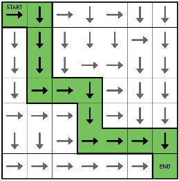
Rather than worry about computing explicit routes between all possible starting location and the goal (an intractable solution at any rate) we can simply leverage reinforcement learning to generate an optimal action from each location that leads to the goal. This type of solution allows for goal navigation from any location on the map which accounts for all the environmental uncertainty up front. At the core, reinforcement learning (RL) is a dressed up Markov decision process (MDP) which is itself a form of discrete-time stochastic control process. Here MDPs provide a mathematical framework for modeling decision making in environments where outcomes are partly random and loosely under the control of a decision maker. MDPs are widely used in optimization problems and solved using dynamic programing (DP) and Bellman’s equation. For more RL content and discussion see previous NVIDIA Developer Blog posts (RL nutshell and OpenAI Gym). Just as MNIST is the iconic deep learning exercise, Gridworld is the classic RL example.
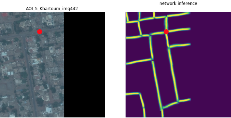
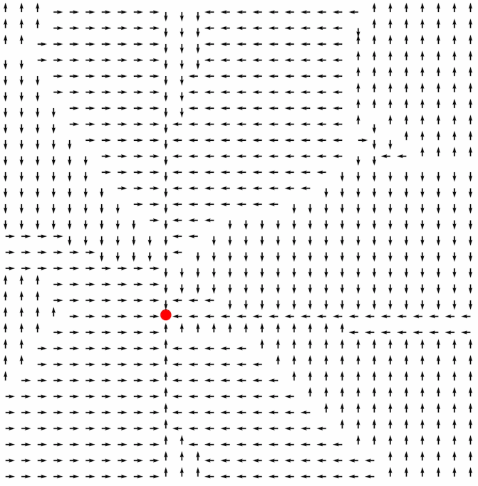
For our application of RL, we will assign some goal state on the road and use the softmax probabilities produced by Mask R-CNN to define the transition probabilities. In a traditional gridworld, there are only four possible actions {up, down, left, right} so that is what we will use for our navigation example here. Notice that even if the neighboring grid location has high value, we discount that value if it leads to a non-traversable location (i.e. low probability of being road). Using simple policy iteration approach (Sutton and Barto, Ch 4) we can determine high-value actions at each grid point which lead to the goal state. One can almost think of this as a coarse vector field that illuminates a force pulling agents in the environment towards to the goal. As a simple example, in Figure 20 below, we consider image 442 from AOI-5 in Khartoum with a goal state in an intersection near the top of the image marked with a large red dot. After a few hundred iterations the optimal policy begins to emerge with clear direction to the goal state (Figure 21 below). Notice that we now have an optimal action for each pixel. Even if the pixel is not a road surface, the policy prescribes the action which leads to the nearest road (i.e. high value areas) and from there to the goal state (obtain maximum reward).
MDPs and RL techniques provide a powerful framework for decision making under uncertainty. Furthermore, these methods can easily accommodate additional environmental information such as buildings (not traversable, must navigate around) and utility functions (i.e. how painful are type I and type II errors), so forth and so on. Additionally, simple policy iteration methods exhibit massive parallelism and can be quickly updated on-the-fly as new information becomes available in an operations or situational awareness type scenario. And finally, this type of decision framework extends naturally to more complex state and reward descriptions to methods such as DeepQ learning (deepRL) and Monte Carlo search trees which led to the historic AlphaGo championship win.
Summary and Closing Comments
In this blog we have presented various methods to model and infer road networks to predict routes between locations within the SpaceNet road detection dataset. This includes experimenting with preprocessing methods to increase model accuracy, using domain knowledge to select the most appropriate spectral bands for a given target of interest, and combining percolation theory and reinforcement learning techniques to calculate navigable and efficient paths directly from imagery.
To enable this we utilized high performance GPU compute resources provided by the NVIDIA GPU Cloud (NGC) and AWS. Using pre-configured NGC framework containers and AMIs eliminated many hours (or days) of setup and provided optimized performance-tuned deep learning frameworks. The Amazon P3 instances provided low-cost easy access to state-of-the-art GPUs for fast network training in just a few hours using the latest NVIDIA Tesla V100 GPUs. Just think, a few years ago this same work would have taken days to configure, tune, debug, and train while costing thousands of dollars for enterprise hardware access. Today with NGC and AWS, we can knock out proof of concept work like this in just hours for around $50. Join us at our GPU Technology Conference 2018 for more great content and the latest in deep learning and artificial intelligence! Use code CMGOV to receive a 25% discount on your GTC registration. See you there!