MLPerf benchmarks are developed by a consortium of AI leaders across industry, academia, and research labs, with the aim of providing standardized, fair, and useful measures of deep learning performance. MLPerf training focuses on measuring time to train a range of commonly used neural networks for the following tasks:
- Natural language processing
- Speech recognition
- Recommender systems
- Biomedical image segmentatione
- Object detection
- Image classification
- Reinforcement learning
Lower training times are important to speed time to deployment, minimizing the total cost of ownership and maximizing return on investment.
However, just as important as a platform’s performance is its versatility. The ability to train every model, as well as provide infrastructure fungibility to run all AI workloads from training to inference, is critical to allowing organizations to maximize return on their infrastructure investments.
The NVIDIA platform, with full-stack innovation and a rich developer and application ecosystem, continues to be the only one to submit results on all eight MLPerf Training tests, as well as to submit on all MLPerf Inference and MLPerf high-performance computing (HPC) tests.
In this post, you will learn about the methods that NVIDIA deployed across the entire stack to deliver more performance in MLPerf v2.0.
Full stack improvements
NVIDIA MLPerf v2.0 submissions are based on the proven A100 Tensor Core GPU, the NVIDIA DGX A100 system, as well as the NVIDIA DGX SuperPOD reference architecture. Many partners also submitted results using the A100 Tensor Core GPU.
Through continued innovation across the entire stack, including system software, libraries, and algorithms, NVIDIA has yet again delivered performance improvements compared to prior submissions using the same A100 Tensor Core GPU.
Compared to NVIDIA MLPerf v0.7 submissions, which marked the first A100 Tensor Core GPU submissions, results showed gains of up to 2.1x on a per-chip basis, and 5.7x for max-scale training (Table 1).
| Benchmark | v2.0 Max-Scale Time to Train (min) (vs. v1.1) (vs. v0.7) | v2.0 Per-Accelerator Time to Train (min) (vs. v1.1) (vs. v0.7) |
| Recommendation (DLRM) | 0.59 (1.08x) (5.66x) | 12.78 (A100) (1.07x) (2.08x) |
| Natural Language Processing (BERT) | 0.21 (1.10x) (4.48x) | 126.95 (A100) (1.26x) (2.69x) |
| Image Classification (ResNet-50 v1.5) | 0.32 (1.09x) (2.38x) | 217.82 (A100) (1.07x) (1.46x) |
| Speech Recognition (RNN-T) | 2.15 (1.10x) (NA*) | 230.07 (A100) (1.19x) (NA*) |
| Image Segmentation (3D U-Net) | 1.22 (1.13x) (NA*) | 170.23 (A100) (1.20x) (NA*) |
| Object Detection – Lightweight (RetinaNet) | 4.25 (NA**) (NA**) | 675.18 (A100) (NA**) (NA**) |
| Object Detection – Heavyweight (Mask R-CNN) | 3.09 (1.05x) (3.39x) | 327.34 (A100) (1.13x) (2.01x) |
| Reinforcement Learning (MiniGo) | 16.23 (0.95x) (1.05x) | 2045.37 (A100) (1.04X) (1.17x) |
MLPerf v1.1 submission details:
Per-Accelerator: BERT: 1.1-2066 | DLRM: 1.1-2064 | Mask R-CNN: 1.1-2066 | Resnet50 v1.5: 1.1-2065 | RNN-T: 1.1-2066 | 3D U-Net: 1.1-2065 | MiniGo: 1.1-2067
Max-Scale: BERT: 1.1-2083 | DLRM: 1.1-2073 | Mask R-CNN: 1.1-2076 | Resnet50 v1.5: 1.1-2082 | SSD: 1.1-2070 | RNN-T: 1.1-2080 | 3D U-Net: 1.1-2077 | MiniGo: 1.1-2081 (*)
MLPerf v2.0 submission details:
Per-Accelerator: BERT: 2.0-2070 | DLRM: 2.0-2068 | Mask R-CNN: 2.0-2070 | Resnet50 v1.5: 2.0-2069 | RetinaNet: 2.0-2091 | RNN-T: 2.0-2066 | 3D U-Net: 2.0-2060 | MiniGo: 2.0-2059
Max-Scale: BERT: 2.0-2106 | DLRM: 2.0-2098 | Mask R-CNN: 2.0-2099 | Resnet50 v1.5: 2.0-2107 | RetinaNet: 2.0-2103 | RNN-T: 2.0-2104 | 3D U-Net: 2.0-2100 | MiniGo: 2.0-2105
Per-Accelerator performance for A100 computed using 8xA100 server time-to-train and multiplying it by 8. 3D U-Net and RNN-T were not part of MLPerf v0.7. (**) RetinaNet was not part of either MLPerf v0.7 or v1.1. MLPerf name and logo are trademarks. For more information, see www.mlperf.org.
The following sections highlight some of the work done to achieve these improvements.
BERT
The latest NVIDIA BERT submission took advantage of the following optimizations:
- Sequence packing
- Fusion of fully connected and GELU layers
Sequence packing
In previous rounds, the overhead related to padding required to fill up the batch was already optimized by introducing an unpadding optimization. Unpadding, however, results in dynamically sized buffers, as the total number of tokens is not fixed anymore.
This is not an issue when we do not have to use CUDA graphs, such when large-batch sizes are used. However, for small batch sizes, where CUDA graphs are used to reduce CPU overhead, dynamically sized buffers require many separate graphs for each possible size. To take advantage of CUDA graphs efficiently while minimizing the overhead of padding, NVIDIA used the concept of sequence packing this round.
In MLPerf Bidirectional Encoder Representations from Transformers (BERT), a training sample has been restricted to 512 tokens, but it often has fewer tokens than 512. As the training sequences have different lengths, it is possible to fit more than one sequence within a 512-token sample.
Sequence packing requires that the length distribution of the training set sequences be known in advance. The sequences can be merged into packed samples such that none of the merged samples exceed a length of 512 tokens.
NVIDIA used a similar packing algorithm that another submitter used in MLPerf v1.1. Adopting an algorithm from a different submitter was made possible by the high degree of general-purpose programmability of GPUs.
To strike a good balance between implementation complexity and performance, up to three sequences were packed in per sample. This results in each training sample containing a varying number of sequences as a batch of three samples can each contain three to nine sequences.
CUDA graphs require buffer sizes to be fixed across time for each graph. The varying number of total sequences was handled by creating a separate graph for each possible number of sequences within a batch.
For large-scale training, we used a batch size of two per chip. This translates into five to seven separate graphs, which is much less than would be required with the unpadding optimization mentioned at the beginning.
Overall, this technique improved the results for large-scale runs by 10% and 33% for 4096-GPU and 1024-GPU scenarios, respectively.
Fusion of fully connected and GELU layers
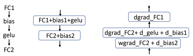
BERT uses a Gaussian error linear unit (GELU) activation function that follows a fully connected layer. In prior submissions, the GELU activation function was implemented as a single kernel. This approach required additional memory transactions for both input reads and output writes.
In this round, NVIDIA implemented the fusion of a fully connected layer (a matrix multiply operation) with the GELU activation function. This eliminated the need for a large number of memory read and write operations, yielding a 2-4% increase in overall throughput – larger gains are observed for larger per-chip batch sizes.
In general, it is more efficient to fuse activation math into the end of matrix multiply operations, which means fusing the GELU activation function into different fully connected layers (Figure 1).
Deep learning recommendation models
The latest NVIDIA deep learning recommendation models (DLRM) submission again leverages NVIDIA Merlin HugeCTR, an optimized open-source deep neural network training framework for recommender systems.
Kernel fusions
Multilayer perceptrons (MLP) represent a key building block for DLRM. To reduce the number of trips to global memory, fusions of elementwise kernels and general matrix multiply (GEMM) kernels have been widely employed.
The NVIDIA cuBLAS library has recently introduced a new fusion type: GEMM with DReLU (fusing ReLU gradient computation with matrix multiply operations in the backward pass). HugeCTR takes advantage of this new fusion type to enhance the performance of MLPs.
Improved overlap of computation and communication
Increasing GPU utilization is important to provide the highest performance.
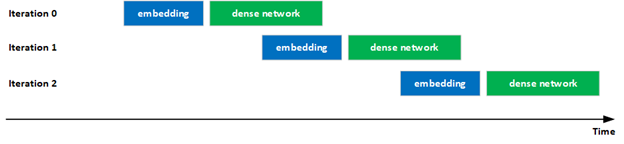
In this latest submission, NVIDIA notably improved the overlap of computations and communications in the evaluation of hybrid embeddings to improve GPU utilization. Specifically, the execution of the dense network in iteration i overlapped with the execution of the embedding in iteration i+1 through pipelining, increasing the utilizations of the GPUs.
This overlapping is possible because there are no inter-iteration dependences in the evaluation phase.
Additionally, several of the key kernels in the forward/backward hierarchical all-to-all operations for hybrid embedding were also optimized.
ResNet-50
For ResNet-50, we employed the following optimizations to boost performance:
- Better max-scale training configuration
- Faster cuDNN kernels
Better max scale training configuration
When a model is trained on a large scale, if the global batch size is not an integer multiple of the training images in the dataset, the last iteration of the epoch gets added extra data to keep the batch size consistent across iterations. This wasted computation can be saved if the global batch size is close to the integer multiple of the dataset. This is especially important for larger-scale training, where the global batch size is relatively large.
In this round of MLPerf, we concluded that using 527 nodes with a global batch size of 67,456 significantly reduced wasted computation, resulting in a performance boost of 3.5% compared to NVIDIA’s ResNet-50 submission in MLPerf v1.1.
Faster CuDNN kernels
For the ResNet50 submission, NVIDIA significantly improved the kernels picked up by cuDNN. This includes both better kernels being picked up for the layer sizes and optimized kernel implementation for different tile sizes.
From these optimized kernel samplings, we observed over 4% throughput improvement in the large-scale configurations from MLPerf v1.1.
RetinaNet
The NVIDIA RetinaNet submission takes advantage of several software optimizations, including:
- Channel last memory format and automatic mixed precision
- Using fusion for speed-up
- Optimizing loss block
- Asynchronous scoring
- CUDA Graphs
Channel last memory format and automatic mixed precision
To avoid memory reorganization and to effectively increase peak performance, NVIDIA used the PyTorch channel last memory format (NHWC instead of NCHW) and the PyTorch automatic mixed precision (AMP).
Using fusion for speed-up
For the RetinaNet submission, NVIDIAtook advantage of several fusion opportunities. The cuDNN runtime fusion through the Apex library was used to fuse CONV-bias-ReLU and CONV-bias patterns, and PyTorch NVFuser were used to fuse element-wise operations, such as scale-bias-ReLU and scale-bias-add-ReLU.
The cuDNN runtime fusion Python interface can be found in the Apex repository (import ConvBiasReLU or ConvBias from apex.contrib.conv_bias_relu).
Optimizing loss block
The RetinaNet loss-related calculations are separated into two stages: ground truth data preprocessing and the actual loss calculation.
As the ground truth data preprocessing is not dependent on the model output, part of the ground truth data processing was offloaded to DALI with custom functions, enabling it to be performed asynchronously, improving system resource utilization. The remainder of the preprocessing was reimplemented and then merged into the model graph to avoid jitter.
For the loss calculation, an optimized focal loss implementation was used, which can be found in the Apex library.
Asynchronous scoring
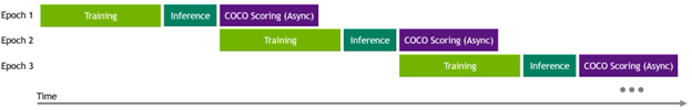
The RetinaNet submission guidelines require that evaluation (inference and scoring) be performed after each training epoch. The scoring time overhead is significant due to the large number of images and bounding boxes in the OpenImages validation dataset, as well as the sequential implementation of the scoring code.
To mitigate the scoring overheads—particularly in large-scale execution, asynchronous scoring was implemented so that the next training epoch masked the previous epoch scoring procedure.
CUDA Graphs
CUDA Graphs were used extensively in the NVIDIA RetinaNet submission. The entire model and portions of the ground truth preprocessing were graphed which required that they be reimplemented to fit CUDA graph constraints.
The model’s forward and backward passes were graph captured, as well as portions of the ground truth preprocessing. The latter required code adaptation to fit CUDA graph constraints.
For more information, see Accelerating PyTorch with CUDA Graphs.
Mask R-CNN
The NVIDIA Mask R-CNN submissions utilized several techniques to improve performance:
- Bottleneck block optimizations
- RPN head fusion
- Evaluation
- Top-K
Bottleneck block optimizations
The resnet backbone is built as a stack of bottleneck blocks, each composed of three sequential convolutions. Each convolution is followed by a batch-norm and a ReLu. The batch-norm modules have four parameters, and some math is required to compute a couple of intermediate terms in the forward method.
As the batch-norms are frozen, the parameters never change, meaning that the intermediate terms do not change either. To save time, these intermediate terms were computed just one time.
Backpropagation of ReLu involves creating and applying a mask. In earlier versions of the code, this mask was stored with half (FP16) precision. In this round, the DReLU mask is represented as a Boolean and not FP16 to reduce memory transactions.
During back propagation, data gradients and weight gradients were computed for each of the three convolution layers. NVIDIA found empirically that while the data gradient GPU kernels were launched with a sufficient number of CTAs to fully use the GPUs, the weight gradient kernels were launched with far fewer CTAs.
One optimization that was implemented was to launch the data gradient kernels first, and then launch all three weight gradient kernels on separate streams so that they ran concurrently. This reduced total computation time for weight gradients.
These optimizations are available for PyTorch users in the bottleneck block module in Apex.
RPN head fusion
A new Apex module, which fuses convolution, bias, and ReLu, was implemented, as discussed in the RetinaNet section. This module was in MaskR-CNN as well to fuse forward propagation of some of the layers in RPN head block.
Evaluation
Evaluation, on average, takes almost as much time as training. Evaluation is done asynchronously on dedicated nodes, but the results are shared with the training nodes through a blocking broadcast.
The training nodes wait for a certain number of steps before they start waiting for the evaluation broadcast to minimize any evaluation result wait time. The learning rate curve has two inflection points in it, and it is extremely unlikely that the model will have converged before passing the last inflection point. That’s why you should wait for as long as possible to check for evaluation results, until training has passed the last learning rate curve inflection point.
Top-K
In earlier versions of PyTorch, the number of CTAs launched by the top-k kernel was proportional to the per-GPU batch size. This yielded poor performance when the batch size equaled 1, the batch size that is always used for NVIDIA max-scale runs.
This issue was addressed in previous rounds with a two-stage top-k method, which was implemented in Python, but this solution did not generalize well. Work on a more general solution was already underway.
In this round, NVIDIA worked with the PyTorch team to ensure that the new top-k implementation that yielded far better performance for a batch size of 1 made it into PyTorch. When this was complete, the prior two-stage top-k implementation was replaced with the new PyTorch module.
3D U-Net
3D U-Net has multiple large layers with an input channel count of 32. For wgrad kernels, using a kernel with the default 64x256x64 meant significant tile size quantization loss.
Thanks to the introduction of the new 32x256x32 wgrad kernels in cuDNN, this tile size quantization loss was saved. This resulted in a speedup of over 5% on a single node in MLPerf v2.0 over MLPerf v1.1.
RNN-T
The preprocessing step of Recurrent Neural Network Transducer (RNN-T) is relatively intensive. Thanks to DALI, most of the preprocessing overhead can be pipelined and hidden under the main training loop.
However, because the size of the input data might vary, there was a need for relocating the internal memory buffers after the initial iteration, increasing the length of the warm-up phase.
DALI has recently switched to a memory-pool based allocator, where the pool is managed using the cuMem API. This significantly reduces the overhead of allocating new buffers, yielding a much faster warm-up process in training.
Conclusion
Thanks to optimizations across the stack, the NVIDIA platform was yet again able to boost performance in MLPerf Training v2.0 using the proven NVIDIA A100 Tensor Core GPU and NVIDIA DGX A100 platforms.
NVIDIA continues to be the only platform to submit results in the MLPerf benchmarking suite, including MLPerf Training, MLPerf Inference, and MLPerf HPC. This showcases the performance and versatility of the entire platform, which is crucial as modern AI becomes pervasive across every computing domain.
In addition to providing the software used for NVIDIA MLPerf submissions in the MLPerf repository, dozens of additional models were also made and optimized for NVIDIA GPUs, available on the NGC hub.
The NVIDIA platform is also ubiquitous, providing customers with the choice of where to run models. NVIDIA A100 is available from all major server makers and cloud service providers, allowing you to deploy on-premises, in the cloud, in a hybrid environment, or at the edge.
