
This post is part of a series on accelerated data analytics.

Because it is generally constrained to a single core, a standard exploratory data analysis (EDA) workflow benefits from accelerated computing with RAPIDS cuDF, an accelerated data analytics library with a pandas-like interface. Time series data notoriously requires additional data processing that adds time and complexity to your workflow, making it another great use case for leveraging RAPIDS.
With RAPIDS cuDF, you can speed up your time series processing for “Goldilocks” datasets that are not too big and not too small. These datasets are onerous on pandas but don’t need full distributed computing tools like Apache Spark or Dask.
What is time series data?
This section covers machine learning (ML) use cases that rely on time series data and when to consider accelerated data processing.
Time series data is ubiquitous. Timestamps are a variable in many types of data sources, from weather measurements and asset pricing to product purchase information and more.
Timestamps come in all levels of granularity, such as millisecond readings or monthly readings. When timestamp data is eventually leveraged in complex modeling, it becomes time series data, indexing the other variables to make patterns observable.
The following prevalent ML use cases rely heavily on time series data, as do many more:
- Anomaly detection for fraud in the financial services industry
- Predictive analytics in the retail industry
- Sensor readings for weather forecasting
- Recommender systems for content suggestions
Complex modeling use cases often require the processing of large datasets with high-resolution historical data that can span years to decades, as well as processing real-time streaming data. Time series data goes through transformations, such as resampling data up and down to make the period of time consistent among datasets and being smoothed into rolling windows that denoise patterns.
pandas provides simple, expressive functions to manage these operations, but you may have observed in your own work that the single-threaded design can quickly get overwhelmed by the amount of processing required. This is especially applicable for larger datasets or use cases that need fast data processing turnaround, which time series–analysis use cases often do. The subsequent wait time for pandas to process the data can be frustrating and can lead to delayed insights.
As a result, these scenarios make cuDF a uniquely good fit for time series data analysis. Using a pandas-like API, you can process tens of gigabytes of data with up to 40x speedups, saving the most valuable asset in any data project: your time.
Time series with RAPIDS cuDF
To showcase the benefit of acceleration for exploring data with RAPIDS cuDF and how it can be readily adopted, this post walks through a subset of time series–processing operations from Time Series Data Analysis. This is a robust notebook analysis of a publicly available dataset of real weather readings, available in the RAPIDS GitHub repository.
In the complete analysis, RAPIDS cuDF executed with a 13x speedup (see the benchmarking section later in this post for exact numbers). Speedups typically increase as the full workflow becomes more complex.
Extrapolating to the real world, this gain has real impact. When an hour-long workload can be completed in under 5 minutes, you can meaningfully add time back to your day.
Dataset
Meteonet is a realistic weather dataset that aggregates readings from weather stations located throughout Paris from 2016-2018, with missing and invalid data. It is about 12.5 GB in size.
Analysis approach
For this post, imagine you are a data scientist who has received this aggregate data for the first time and must prepare this for a meteorological use case. The specific use case is open-ended: it could be a forecast, report, or input in a climate model.
As you review this post, most of the functions should be familiar as they are designed to resemble operations in pandas. This analysis is structured to perform the following tasks:
- Format the DataFrame.
- Resample the time series.
- Run a rolling-window analysis.
This post disregards several data inconsistencies that are addressed in the end-to-end workflow demonstrated in the notebook, Time Series Data Analysis Using cuDF.
Step 1. Format the DataFrame
First, import the packages used in this analysis with the following command:
# Import the necessary packages
import cudf
import cupy as cp
import pandas as pd
Next, read in the CSV data.
## Read in data
gdf = cudf.read_csv('./SE_data.csv')
Begin by focusing on the meteorological parameters of interest: wind speed, temperature, and humidity.
gdf = gdf.drop(columns=['dd','precip','td','psl'])After the parameters of interest are isolated, perform a series of quick checks. Start the first transformation by converting the date column to the datetime data type. Then, print out the first five rows to visualize what you are working with and assess the size of the tabular dataset.
# Change the date column to the datetime data type. Look at the DataFrame info
gdf['date'] = cudf.to_datetime(gdf['date'])
gdf.head()
Gdf.shape| number_sta | lat | lon | height_sta | date | ff | hu | t | |
| 0 | 1027003 | 45.83 | 5.11 | 196.0 | 2016-01-01 | <NA> | 98.0 | 279.05 |
| 1 | 1033002 | 46.09 | 5.81 | 350.0 | 2016-01-01 | 0.0 | 99.0 | 278.35 |
| 2 | 1034004 | 45.77 | 5.69 | 330.0 | 2016-01-01 | 0.0 | 100.0 | 279.15 |
| 3 | 1072001 | 46.20 | 5.29 | 260.0 | 2016-01-01 | <NA> | <NA> | 276.55 |
| 4 | 1089001 | 45.98 | 5.33 | 252.0 | 2016-01-01 | 0.0 | 95.0 | 279.55 |
Output
The DataFrame shape (127515796, 8) shows 127,515,796 rows by eight columns. Now that the size and shape of the dataset are known, you can start investigating a bit deeper to see how frequently the data is sampled.
## Investigate the sampling frequency with the diff() function to calculate the time diff
## dt.seconds, which is used to find the seconds value in the datetime frame. Then apply the
## max() function to calculate the maximum date value of the series.
delta_mins = gdf['date'].diff().dt.seconds.max()/60
print(f"The dataset collection covers from {gdf['date'].min()} to {gdf['date'].max()} with {delta_mins} minute sampling interval")
The dataset covers sensor readings from 2016-01-01T00:00:00.000000000 to 2018-12-31T23:54:00.000000000, at a 6-minute sampling interval. Confirm that the dates and times expected are represented in the dataset.
After a basic review of the dataset is complete, get started with time series-specific formatting. Begin by separating the time increments into separate columns.
gdf['year'] = gdf['date'].dt.year
gdf['month'] = gdf['date'].dt.month
gdf['day'] = gdf['date'].dt.day
gdf['hour'] = gdf['date'].dt.hour
gdf['mins'] = gdf['date'].dt.minute
gdf.tail
The data is now separated into columns at the end for year, month, and day. This makes slicing the data by different increments much simpler.
| number_sta | lat | lon | height_sta | date | ff | hu | t | year | month | day | hour | mins | |
| 127515791 | 84086001 | 43.811 | 5.146 | 672.0 | 2018-12-31 23:54:00 | 3.7 | 85.0 | 276.95 | 2018 | 12 | 31 | 23 | 54 |
| 127515792 | 84087001 | 44.145 | 4.861 | 55.0 | 2018-12-31 23:54:00 | 11.4 | 80.0 | 281.05 | 2018 | 12 | 31 | 23 | 54 |
| 127515793 | 84094001 | 44.289 | 5.131 | 392.0 | 2018-12-31 23:54:00 | 3.6 | 68.0 | 280.05 | 2018 | 12 | 31 | 23 | 54 |
| 127515794 | 84107002 | 44.041 | 5.493 | 836.0 | 2018-12-31 23:54:00 | 0.6 | 91.0 | 270.85 | 2018 | 12 | 31 | 23 | 54 |
| 127515795 | 84150001 | 44.337 | 4.905 | 141.0 | 2018-12-31 23:54:00 | 6.7 | 84.0 | 280.45 | 2018 | 12 | 31 | 23 | 54 |
Experiment with the updated DataFrame by selecting a specific time range and station to analyze.
# Use the cupy.logical_and(...) function to select the data from a specific time range.
import pandas as pd
start_time = pd.Timestamp('2017-02-01T00')
end_time = pd.Timestamp('2018-11-01T00')
station_id = 84086001
gdf_period = gdf.loc[cp.logical_and(cp.logical_and(gdf['date']>start_time,gdf['date']<end_time),gdf['number_sta']==station_id)]
gdf_period.shape
(146039, 13)
The DataFrame has been successfully prepared, with 13 variables and 146,039 rows.
Step 2. Resample the time series
Now that the DataFrame has been set up, run a simple resampling operation. Although the data updates every 6 minutes, in this case, the data must be reshaped to fall into a daily cadence.
First set the date as the index, so that the rest of the variables adjust as time does. Downsample the data from samples every 6 minutes to one record per day, to yield one record for each variable on each day. Retain the maximum value of each variable for each day as the record for that day.
## Set "date" as the index. See what that does?
gdf_period.set_index("date", inplace=True)
## Now, resample by daylong intervals and check the max data during the resampled period.
## Use .reset_index() to reset the index instead of date.
gdf_day_max = gdf_period.resample('D').max().bfill().reset_index()
gdf_day_max.head()
The data is now available in daily increments. Refer to the table as a check that the operation yielded the desired result.
| date | number_sta | lat | lon | height_sta | ff | hu | t | year | month | day | hour | mins | |
| 0 | 2017-02-01 | 84086001 | 43.81 | 5.15 | 672.0 | 8.1 | 98.0 | 283.05 | 2017 | 2 | 1 | 23 | 54 |
| 1 | 2017-02-02 | 84086001 | 43.81 | 5.15 | 672.0 | 14.1 | 98.0 | 283.85 | 2017 | 2 | 2 | 23 | 54 |
| 2 | 2017-02-03 | 84086001 | 43.81 | 5.15 | 672.0 | 10.1 | 99.0 | 281.45 | 2017 | 2 | 3 | 23 | 54 |
| 3 | 2017-02-04 | 84086001 | 43.81 | 5.15 | 672.0 | 12.5 | 99.0 | 284.35 | 2017 | 2 | 4 | 23 | 54 |
| 4 | 2017-02-05 | 84086001 | 43.81 | 5.15 | 672.0 | 7.3 | 99.0 | 280.75 | 2017 | 2 | 5 | 23 | 54 |
Step 3. Run a rolling-window analysis
In the previous resampling example, points are sampled based on time. However, you can also smooth data based on frequency, using a rolling window.
In the following example, take a rolling window of length three over the data. Again, retain the maximum value for each variable.
# Specify the rolling window.
gdf_3d_max = gdf_day_max.rolling('3d',min_periods=1).max()
gdf_3d_max.reset_index(inplace=True)
gdf_3d_max.head()
Rolling windows can be used to denoise data and assess data stability over time.
| date | number_sta | lat | lon | height_sta | ff | hu | t | year | month | day | hour | mins | |
| 0 | 2017-02-01 | 84086001 | 43.81 | 5.15 | 672.0 | 8.1 | 98.0 | 283.05 | 2017 | 2 | 1 | 23 | 54 |
| 1 | 2017-02-02 | 84086001 | 43.81 | 5.15 | 672.0 | 14.1 | 98.0 | 283.85 | 2017 | 2 | 2 | 23 | 54 |
| 2 | 2017-02-03 | 84086001 | 43.81 | 5.15 | 672.0 | 14.1 | 99.0 | 283.85 | 2017 | 2 | 3 | 23 | 54 |
| 3 | 2017-02-04 | 84086001 | 43.81 | 5.15 | 672.0 | 14.1 | 99.0 | 283.35 | 2017 | 2 | 4 | 23 | 54 |
| 4 | 2017-02-05 | 84086001 | 43.81 | 5.15 | 672.0 | 12.5 | 99.0 | 283.35 | 2017 | 2 | 5 | 23 | 54 |
This post walked you through the common steps of time series data processing. While a weather dataset was used for the example, the steps are applicable to all forms of time series data. The process is similar to your time series analysis code today.
Performance speedup
When running through the complete notebook with the Meteonet weather dataset, we achieved a 13x speedup on an NVIDIA RTX A6000 GPU using RAPIDS 23.02 (Figure 1).
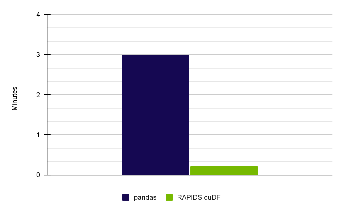
| Pandas on CPU (Intel Core i7-7800X CPU) | User: 2 min 32 sec Sys: 27.3 sec Total: 3 min |
| RAPIDS cuDF on NVIDIA A6000 GPUs | User: 5.33 sec Sys: 8.67 sec Total: 14 sec |
Key takeaways
Time series analysis is a core part of analytics that requires additional processing compared to other variables. With RAPIDs cuDF, you can manage the processing step faster and reduce time to insight with the Pandas functions you are accustomed to.
To further investigate cuDF in time series analysis, see rapidsai-community/notebooks-contrib on GitHub. To revisit cuDF in EDA applications, see Accelerated Data Analytics: Speed Up Data Exploration with RAPIDS cuDF.
Register for NVIDIA GTC 2023 for free and join us March 20–23 for related data science sessions.
Acknowledgments
Meiran Peng, David Taubenheim, Sheng Luo, and Jay Rodge contributed to this post.
