
This post is part of a series on accelerated data analytics.
Digital advancements in climate modeling, healthcare, finance, and retail are generating unprecedented volumes and types of data. IDC says that by 2025, there will be 180 ZB of data compared to 64 ZB in 2020, scaling up the need for data analytics to turn all that data into insights.
- Incoming satellite images twice a day are informing air quality, flooding, and solar flares modeling to help discern natural risks.
- Advanced genomics and gene sequencing provide pools of genetic data encoded with insights that can bring us closer to a cure for cancer.
- Digital purchase and networking systems are producing terabytes of market and behavioral data.
NVIDIA provides the RAPIDS suite of open-source software libraries and APIs to give data scientists the ability to execute end-to-end data science and analytics pipelines entirely on GPUs. This includes common data preparation tasks for analytics and data science with our DataFrame API: RAPIDS cuDF.
With speed-ups of up to 40x in typical data analytics workflows, accelerated data analytics saves you time and adds opportunities for iteration that may be constrained by your current analytics tools.
To explain the value of accelerated data analytics, we walk through a simple exploratory data analysis (EDA) tutorial using RAPIDS cuDF in this post.
If you’re using Spark 3.0 today to process large datasets, see the RAPIDS accelerator for Spark. If you are ready to get started with RAPIDS now, see Step-by-Step Guide to Building a Machine Learning Application with RAPIDS.
Why RAPIDS cuDF for EDA?
Today, most data scientists use pandas, the popular open-source software library built on top of Python specifically for data manipulation and analysis for EDA tasks. Its flexible and expressive data structures are designed to make working with relational or labeled data both easy and intuitive, especially for open-ended workflows like EDA.
However, pandas is designed to run on a single core and starts slowing down when data size hits 1-2 GB, limiting its applicability. If the data size exceeds the 10-20 GB range, distributed computing tools like Dask and Apache Spark should be considered. The downside is that they require code rewrites that can be a barrier to adoption.
For that middle ground of 2-10 GB, RAPIDS cuDF is the Goldilocks solution that is just right.
RAPIDS cuDF parallelizes compute to multiple cores in the GPU, and is abstracted into a pandas-like API. With cuDF functions that mimic many of the most popular and standard operations in pandas, cuDF runs like pandas but faster. Think of RAPIDS as a turbo boost button for your current pandas workloads.
EDA with RAPIDS cuDF
This post demonstrates how easy cuDF is to adopt when taking an EDA approach.
With the operations covered in this post, we observed a 15x speedup in operations when using cuDF, compared to pandas. This modest gain can help you save time when working on multiple projects.
For more information about conducting time series analysis, see the full notebook, Exploratory Data Analysis Using cuDF, in the RAPIDS GitHub repository. The speedup observed increases to 15x with the full workflow.
Dataset
Meteonet is a weather dataset that aggregates readings from weather stations located throughout Paris from 2016-2018. It is a realistic dataset, with missing and invalid data.
Analysis approach
For this post, imagine that you are a data scientist reading this aggregate data and assessing its qualities. The use case is open-ended; the readings could be used for reports, a weather forecast, or to inform civil engineering use cases.
Structure your analysis to contextualize the data by the following steps:
- Understanding the variables.
- Identifying the gaps in the dataset.
- Analyzing the relationships between variables.
Step 1. Understand the variables
First, import the cuDF library and read in the dataset. To download and create NW.csv, which contains data for 2016, 2017, and 2018 for northwest stations, see the Exploratory Data Analysis Using cuDF notebook.
# Import cuDF and CuPy
import cudf
import cupy as cp

# Read in the data files into DataFrame placeholders
gdf_2016 = cudf.read_csv('./NW.csv')
Review the dataset and understand the variables that you are working with. This helps you understand the dimensions of and the kinds of data in the DataFrame. There’s a similarity to pandas syntax throughout.
Look at the overall DataFrame structure, using the .info command, which is the same in pandas:
GS_cudf.info()
<class 'cudf.core.dataframe.DataFrame'>
RangeIndex: 22034571 entries, 0 to 22034570
Data columns (total 12 columns):
 #   Column      Dtype
---  ------      -----
 0   number_sta  int64
 1   lat         float64
 2   lon         float64
 3   height_sta  float64
 4   date        datetime64[ns]
 5   dd          float64
 6   ff          float64
 7   precip      float64
 8   hu          float64
 9   td          float64
 10  t           float64
        object
dtypes: datetime64[ns](1), float64(9), int64(1), object(1)
memory usage: 6.5+ GB
From the output, there are 12 variables observed, and you can see their titles.
To get further into the data, determine the overall shape of the DataFrame: rows by columns.
# Checking the DataFrame dimensions. Millions of rows by 12 columns.
GS_cudf.shape
(65826837, 12)
At this point, the dataset dimensions are known, but each variable’s data range is unknown. As there are 65,826,837 rows, you cannot visualize the whole dataset at one time.
Instead, look at the first five rows of the DataFrame to examine the variable inputs in a consumable sample:
# Display the first five rows of the DataFrame to examine details
GS_cudf.head()
| number_sta | lat | lon | height_sta | date | dd | ff | precip | hu | td | t | psl | |
| 0 | 14066001 | 49.33 | -0.43 | 2.0 | 2016-01-01 | 210.0 | 4.4 | 0.0 | 91.0 | 278.45 | 279.85 | <NA> |
| 1 | 14126001 | 49.15 | 0.04 | 125.0 | 2016-01-01 | <NA> | <NA> | 0.0 | 99.0 | 278.35 | 278.45 | <NA> |
| 2 | 14137001 | 49.18 | -0.46 | 67.0 | 2016-01-01 | 220.0 | 0.6 | 0.0 | 92.0 | 276.45 | 277.65 | 102360.0 |
| 3 | 14216001 | 48.93 | -0.15 | 155.0 | 2016-01-01 | 220.0 | 1.9 | 0.0 | 95.0 | 278.25 | 278.95 | <NA> |
| 4 | 14296001 | 48.80 | -1.03 | 339.0 | 2016-01-01 | <NA> | <NA> | 0.0 | <NA> | <NA> | 278.35 | <NA> |
Table 1. Output results
You can get an idea of what each row contains now. How many sources of data are there? Look at the number of stations gathering all this data:
# How many weather stations are covered in this dataset?
# Call nunique() to count the distinct elements along a specified axis.

number_stations = GS_cudf['number_sta'].nunique()
print("The full dataset is composed of {} unique weather stations.".format(GS_cudf['number_sta'].nunique()))
The full dataset is composed of 287 unique weather stations. How frequently do these stations update their data?
## Investigate the frequency of one specific station's data
## date column is datetime dtype, and the diff() function calculates the delta time
## TimedeltaProperties.seconds can help get the delta seconds between each record, divide by 60 seconds to see the minutes difference.
delta_mins = GS_cudf['date'].diff().dt.seconds.max()/60
print(f"The data is recorded every {delta_mins} minutes")
The data is recorded every 6.0 minutes. The weather stations produce 10 records an hour.
Now, you understand the following data characteristics:
- Data types
- Dimensions of the dataset
- Number of sources garnering the dataset
- Dataset update frequency
However, you must still explore whether this data has major gaps, either with missing or invalid data inputs. These issues affect whether this data can be used as a reliable source on its own.
Step 2. Identify the gaps
These weather stations have multiple sensors. Any single sensor could have gone down or provided an unreliable reading throughout the year. Some missing data is acceptable, but if the stations went down too often, the data could be misrepresentative of true conditions throughout the year.
To understand the reliability of this data source, analyze the rate of missing data and the number of invalid inputs.
To evaluate the rate of missing data, compare the number of readings to the expected number of readings.
The dataset includes 271 unique stations, with 10 records entered per hour (one every 6 minutes). The expected number of recorded data entries, assuming no downtime of sensors, is 271 x 10 x 24 x 365 = 23,739,600. But, as observed earlier from the .shape operation, you have only 22,034,571 rows of data.
# Theoretical number of records is...
theoretical_nb_records = number_stations * (60 / delta_mins) * 365 * 24
actual_nb_of_rows = GS_cudf.shape[0]
missing_record_ratio = 1 - (actual_nb_of_rows/theoretical_nb_records)
print("Percentage of missing records of the NW dataset is: {:.1f}%".format(missing_record_ratio * 100))
print("Theoretical total number of values in dataset is: {:d}".format(int(theoretical_nb_records)))

Percentage of missing records of the NW dataset is: 12.7%
When contextualizing the full year, 12.7% represents about ~19.8 weeks of missing data per year.
You know that around 5 months of data out of 36 was simply not recorded. For other data points, you have some missing data, where recordings are made for some variables but not for others. You saw this when you looked at the first five rows of the dataset, which contain NAs.
To understand how much NA data you have, start by identifying which variables have NA readings. Assess how many invalid readings each category has. Cut the dataset down to consider only 2018 data for this part of the analysis.
# Finding which items have NA value(s) during year 2018
NA_sum = GS_cudf[GS_cudf['date'].dt.year==2018].isna().sum()
NA_data = NA_sum[NA_sum>0]
NA_data.index

StringIndex(['dd' 'ff' 'precip' 'hu' 'td' 't' 'psl'], dtype='object')
NA_data
dd         8605703
ff         8598613
precip     1279127
hu         8783452
td         8786154
t          2893694
psl       17621180
dtype: int64
You can see that PSL (sea level pressure) has the highest number of missing readings. Around ~80% of its total readings are not recorded. On the low end, precipitation has ~6% invalid readings, which indicates that the sensor is robust.
These two indicators help you understand where gaps exist in the dataset and which parameters to rely on during analysis. For a comprehensive analysis of how data validity changes each month, see the notebook.
Now that you have a good grasp of what the data looks like and its gaps, you can look at relationships between variables that could affect the statistical analysis.
Step 3. Analyze the relationship between variables
All ML applications rely on statistical modeling, as well as many analytics applications. For any use case, be aware of the variables that are highly correlated, as they could skew results.
For this post, analyzing the readings from the meteorological categories is the most relevant. Generate a correlation matrix for the full 3-year dataset to assess any dependencies to be aware of.
# Only analyze meteorological columns
Meteo_series = ['dd', 'ff', 'precip' ,'hu', 'td', 't', 'psl']
Meteo_df = cudf.DataFrame(GS_cudf,columns=Meteo_series)
Meteo_corr = Meteo_df.dropna().corr()

# Check the items with correlation value > 0.7
Meteo_corr[Meteo_corr>0.7]
| dd | ff | precip | hu | td | t | psl | |
| dd | 1.0 | <NA> | <NA> | <NA> | <NA> | <NA> | <NA> |
| ff | <NA> | 1.0 | <NA> | <NA> | <NA> | <NA> | <NA> |
| precip | <NA> | <NA> | 1.0 | <NA> | <NA> | <NA> | <NA> |
| hu | <NA> | <NA> | <NA> | 1.0 | <NA> | <NA> | <NA> |
| td | <NA> | <NA> | <NA> | <NA> | 1.0 | 0.840558357 | <NA> |
| t | <NA> | <NA> | <NA> | <NA> | 0.840558357 | 1.0 | <NA> |
| psl | <NA> | <NA> | <NA> | <NA> | <NA> | <NA> |
In the matrix, there is a significant correlation between td (dew point) and t (temperature). Take this into account if you are using any future algorithm that assumes the variables are independent, such as linear regression. You can go back to the invalid data analysis to see if one has more missing readings than the other as a metric to select.
After a basic exploration, you now understand the data’s dimension and variables and have reviewed a variable correlation matrix. There are many more EDA techniques, but the method in this post is generic with a typical set of starting points that any data scientist would be familiar with. As you saw throughout the tutorial, cuDF is near-identical to pandas syntax.
Benchmarking RAPIDS cuDF for EDA
As previously mentioned, this post is a simplified walkthrough of the complete workflow in the full notebook. For this post, we observed a 9.55x speedup. These results were achieved on an NVIDIA A6000 GPU.
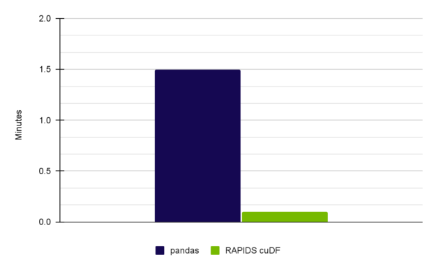
Table 3 shows a performance comparison, with results from this post and the full notebook.
|
Full Notebook (15x speed-up) |
Pandas on CPU (Intel Core i7-7800X CPU) |
user 1 min 15 sec sys: 14.3 sec total: 1 min 30 sec |
|
RAPIDS cuDF on NVIDIA A6000 |
user 3.92 sec sys: 2.03 sec total: 5.95 sec |
Table 3. A 15x speedup was achieved for EDA performed with RAPIDS cuDF on an NVIDIA RTX A6000 GPU
Key takeaways
Realistic data from live sources has gaps, missing information, and correlations that have to be addressed before you model it to develop insights.
With the observed speed-up of 15x, you can extrapolate your time saved for a longer, more complex workload. If it takes 1 hour to run EDA steps, you can complete that effort in 4 minutes. That leaves you with 56 minutes to address unforeseen issues in the data, complete data processing, add another year’s worth of data to this set to minimize gaps, and begin engineering the dataset to fit your use case. Best of all, you can regain control of your time.
To further investigate cuDF in exploratory data analysis, review the full notebook, Exploratory Data Analysis Using cuDF. Register for NVIDIA GTC 2023 for free and join us March 20–23 for related data science sessions.
To see cuDF in action with time series data, see Accelerated Data Analytics: Faster Time Series Analysis with RAPIDS cuDF.
Acknowledgments
Meiran Peng, David Taubenheim, Sheng Luo, and Jay Rodge contributed to this post.
