This is the third installment of the series of introductions to the RAPIDS ecosystem. The series explores and discusses various aspects of RAPIDS that allow its users solve ETL (Extract, Transform, Load) problems, build ML (Machine Learning) and DL (Deep Learning) models, explore expansive graphs, process geospatial, signal, and system log data, or use SQL language via BlazingSQL to process data.
We are living in a world surrounded by data. The massive amount of information flowing through the wires nowadays is mind-boggling and the amount of compute power necessary to process and store this data is equally outrageous. Rarely these days we have data that fits on a single machine unless for prototyping.

Accelerate GPU data processing with Dask
The solution: use more machines. Distributed data processing frameworks have been available for at least 15 years as Hadoop was one of the first platforms built on the MapReduce paradigm introduced by Google. In 2012, unsatisfied with the performance of Hadoop, initial versions of Apache Spark were released. Spark has grown to become the leading platform for processing data using SQL and DataFrames in memory.
However, both of these frameworks use somewhat esoteric languages for Data Science making it challenging to quickly switch from R or Python. This has changed in 2015 when version 0.2.0 of Dask was released and has quickly become a major player in the distributed PyData ecosystem. RAPIDS uses Dask to scale computations on NVIDIA GPUs to clusters of hundreds or thousands of GPUs.
The previous tutorials in the series showcased other areas:
- In the first post, Python pandas tutorial we introduced cuDF, the RAPIDS DataFrame framework for processing large amounts of data on an NVIDIA GPU.
- The second post, compared similarities between cuDF DataFrame and pandas DataFrame.
In this tutorial, we will introduce Dask, a Python distributed framework that helps to run distributed workloads on CPUs and GPUs. To help with getting familiar with Dask, we also published Dask4Beginners-cheatsheets that can be downloaded here.
Distributed paradigm
We live in a massively distributed yet interconnected world. Daily, a colossal amount of information circles the globe, and people use the relevant bits to drive decisions. With the world’s progress and increased data production, the data assembly line had to adapt.
Distributed systems rely on the fact that the data does not sit on a single machine (where the data process can access it) but is distributed among many machines (with some replication strategy). Since data is distributed, to process it, we only need to ship instructions to inform a worker process running on a machine that is part of a cluster to execute it. Depending on the execution graph, each machine in the cluster either stores the intermediate results for further processing or returns the computed results to the head-node (also known as the scheduler) running a scheduler process for final results assembly.
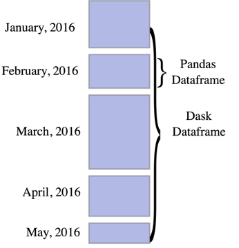
A data partition is the part of the dataset that is local to a worker process, and various chunks of the dataset are replicated across the cluster. This ensures that should any of the worker processes fail or exit the cluster, the data processing will not fail as the same data part can be processed by other workers.
Dask
Dask partitions data (even if running on a single machine). However, in the case of Dask, every partition is a Python object: it can be a NumPy array, a pandas DataFrame, or, in the case of RAPIDS, a cuDF DataFrame.

Unlike Hadoop, which requires users to build the entire pipeline from scratch (and save the intermediate results to disk), and unlike Spark that makes it relatively hard to build execution graphs, Dask provides the data types (like DataFrames) that abstract most of the processing. Dask data types are feature-rich and provide the flexibility to control the task flow should users choose to.
Cluster and client
To start processing data with Dask, users do not really need a cluster: they can import dask_cudf and get started. However, creating a cluster and attaching a client to it gives everyone more flexibility. And it is not as scary as it sounds and users can get the cluster and client up and running with 4 lines of code.
from dask_cuda import LocalCUDACluster
from dask.distributed import Client
cluster = LocalCUDACluster()
client = Client(cluster)
The client is now running on a cluster that has a single worker (a GPU).
Processing data
Many ways exist to create a Dask cuDF DataFrame. However, if users already have a cuDF DataFrame, they can convert it to run distributedly.
ddf = dask_cudf.from_cudf(df, npartitions=2)
Of course, Dask cuDF can also read many data formats (CSV/TSC, JSON, Parquet, ORC, etc) and while reading even a single file user can specify the chunksize so each partition will have the same size.
A very powerful feature of Dask cuDF DataFrames is its ability to apply the same code one could write for cuDF with a simple cuDF with a map_partitions wrapper. Here is an extremely simple example of a cuDF DataFrame:
df['num_inc'] = df['number'] + 10
We take the number column and add 10 to it. With Dask cuDF DataFrame in a very similar fashion:
ddf['num_inc'] = df['number'] + 10
Not transformations can be fit within this paradigm though. A more elegant and universal solution would be to use the same code used to process cuDF DataFrame and wrap it within a map_partitions call:
def process_frame(df):
    df['num_inc'] = df['number'] + 10
    return df

ddf.map_partitions(process_frame)
If there is any feature that is available in cuDF but not yet supported by Dask cuDF, then this a way to still process your data: since under the hood Dask cuDF objects are simply cuDF DataFrames, what map_partitions call does is it runs the specified code or functions on the underlying cuDF DataFrame rather than applying the transformation to the Dask cuDF DataFrame. This way, even more sophisticated processing can be achieved and makes the code more readable, maintainable, and reusable.
def divide(a, div, b):
    for i, aa in enumerate(a):
        div[i] = aa / b

def process_frame_div(df, col_a, val_divide):
    df = df.apply_rows(
        divide
        , incols = {col_a: 'a'}
        , outcols = {'div': np.float64}
        , kwargs = {'b': val_divide}
    )

    return df['div']

ddf['div_number'] = ddf.map_partitions(process_frame_div, 'number', 10.0)
ddf['div_float']  = ddf.map_partitions(process_frame_div, 'float_number', 5.0)
In this example, we not only use a custom CUDA kernel to process our data but also pass parameters to the map_partitions function so we can reuse the same logic to process multiple columns.
Lazy execution
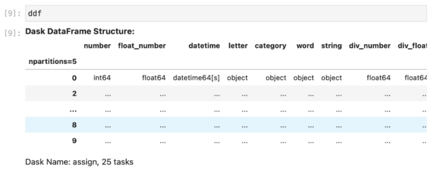
Now, if we try to peek inside the ddf DataFrame, we will most likely see a view similar to this one:

This means that the data has not been processed in any way yet.
Dask employs the lazy execution paradigm: rather than executing the processing code instantly, Dask builds a Directed Acyclic Graph (DAG) of execution instead; DAG contains a set of tasks and their interactions that each worker needs to execute. However, the tasks do not run until the user tells Dask to execute them in one way or another. With Dask users have three main options:
- Call
compute() on a DataFrame. This call will process all the partitions and then return results to the scheduler for final aggregation and conversion to cuDF DataFrame. This should be used sparingly and only on heavily reduced results unless your scheduler node runs out of memory. - Call
persist() on a DataFrame. This call executes the graph but instead of returning the results to the scheduler node, it persists them across the cluster in memory so the user can reuse these intermediate results down the pipeline without the need of rerunning the same processing. - Call
head() on a DataFrame. Just like with cuDF, this call will return 10 records back to the scheduler node.
So, unless the user calls either of these actions the workers will sit idle waiting for the scheduler to initiate the processing.
This is just the tip of the iceberg of Dask’s capabilities. To find out about other functionality of Dask, download the handy Dask for beginners cheat sheet!
