Deep learning is achieving significant success in various fields and areas, as it has revolutionized the way we analyze, understand, and manipulate data. There are many success stories in computer vision, natural language processing (NLP), medical diagnosis and health care, autonomous vehicles, recommendation systems, and climate and weather modeling.
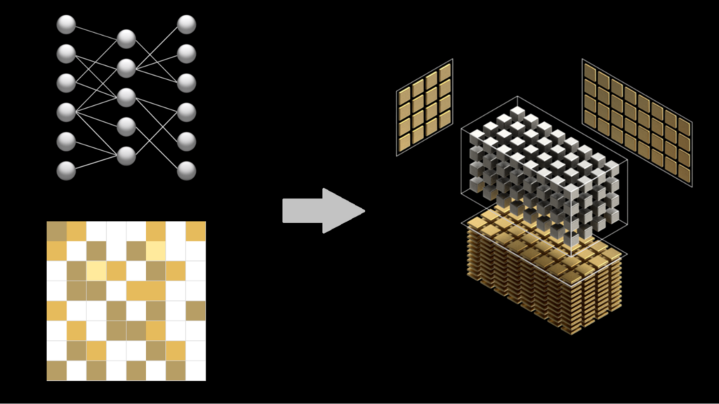
In an era of ever-growing neural network models, the high demand for computational speed becomes a big challenge for hardware and software. Model pruning and low-precision inference are useful solutions.
Starting with the NVIDIA Ampere architecture and the introduction of the A100 Tensor Core GPU, NVIDIA GPUs have the fine-grained structured sparsity feature, which can be used to accelerate inference. For more information, see the NVIDIA A100 Tensor Core GPU Architecture: Unprecedented Acceleration at Every Scale whitepaper.
In this post, we introduce some training recipes for such sparse models to maintain accuracy, including the basic recipes, the progressive recipes, and the combination with int8 quantization. We also discuss how to do the inference with the structured sparsity in the NVIDIA Ampere architecture.
Tencent’s Machine Learning Platform department (MLPD) used the progressive training techniques to simplify training and achieve better accuracy. With the sparsity feature and some quantization techniques, they achieved 1.3–1.8x acceleration in Tencent’s offline services.
Structured sparsity in the NVIDIA Ampere architecture
NVIDIA Ampere and NVIDIA Hopper architecture GPUs add the new feature of fine-grained structured sparsity, which can mainly be used to accelerate inference workloads. This feature is supported by sparse Tensor Cores, which require a 2:4 sparsity pattern. Among each group of four contiguous values, at least two must be zero, which is a 50% sparsity rate.
This pattern can have efficient memory access, good speedup, and can easily recover accuracy. After compression, only non-zero values and the associated index metadata are stored (Figure 1). The sparse Tensor Cores process only the non-zero values when doing matrix multiplication and theoretically, the compute throughput would be 2x compared to the equivalent dense matrix multiplication.
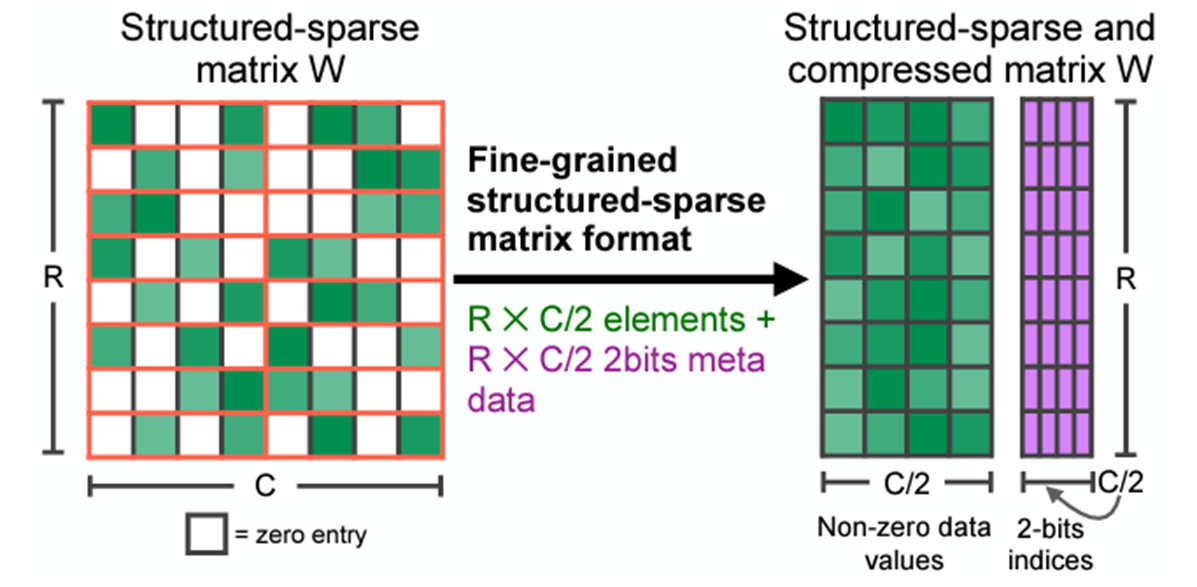
Structured sparsity can mainly be applied on fully connected layers and convolution layers where 2:4 sparse weights are provided. If you prune the weights of these layers in advance, then these layers can be accelerated by structured sparsity.
Training recipes
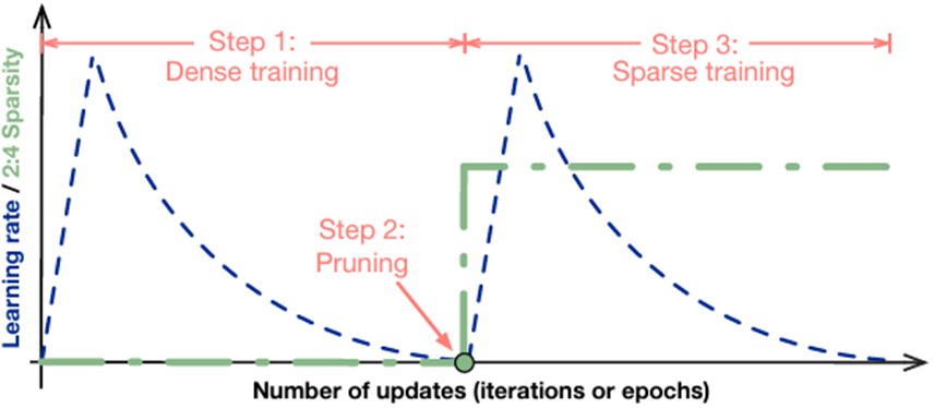
As directly pruning the weights decreases the model accuracy, you should do some training to recover the accuracy when using the structured sparsity. Here, we introduce some basic recipes and new progressive recipes.
Basic recipes
The basic recipes maintain the model accuracy without any hyperparameter tuning. For more information, see Accelerating Sparse Deep Neural Networks.
The workflow is easy to follow:
- Train a model without sparsity.
- Prune the model in a 2:4 sparse pattern for the FC and convolution layers.
- Retrain the pruned model by following these rules:
- Initialize the weights to the values from Step 2.
- Use the same optimizer and hyperparameter (learning rate, schedule, number of epochs, and so on) as in Step 1.
- Maintain the sparsity pattern computed in Step 2.
There are also some advanced recipes for complicated cases.
For example, apply sparse training in multiple stages. For some object detection models, if the dataset in the downstream task is large enough, you can just repeat the fine-tuning with sparsity. For models like BERT-SQuAD, the dataset is relatively small, and you must apply the sparsity to the pretraining phase for better accuracy.
Also, you can easily combine the sparsity training with int8 QAT by inserting the quant nodes before fine-tuning. All these training and fine-tuning methods are one-shot, as the final model is obtained after one sparse training process.
Progressive training recipes
One-shot sparse fine-tuning can cover most tasks and achieve speedup without accuracy loss. On the other hand, for some difficult tasks that are sensitive to weight changes, one-shot sparsity for all weights causes large information loss. It’s difficult to recover accuracy by only fine-tuning with small datasets, and sparse pretraining is also needed for these tasks.
Sparse pretraining requires more data and is more time-consuming. So, inspired by the pruning method for CNN, the progressive sparsity is introduced to apply sparsity only on fine-tuning phase for such tasks without too much accuracy loss. For more information, see Learning Both Weights and Connections for Efficient Neural Networks.

The key idea of progressive sparsity is to divide the target sparsity ratio into several small steps.
\(S_{target} = \sum\limits_{n-1}^{N} S_n\)
As shown in the equation and Figure 4, for a target sparsity ratio S, you divide it into N steps, which facilitates the rapid recovery of information during the fine-tuning process. Based on our experiments, progressive sparsity can achieve higher accuracy than one-shot sparsity with the same fine-tuning epochs.
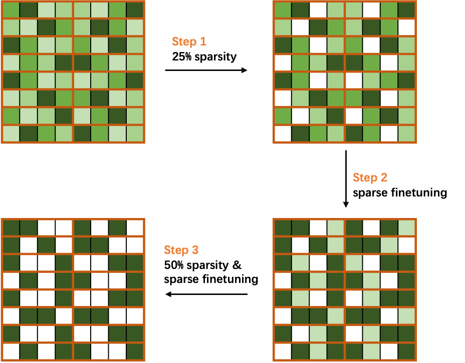
Taking 50% sparsity in a 2:4 pattern as a simple case, divide the sparsity ratio into two steps, and progressively sparse and fine-tune the weights in the network.
As shown in Figure 4, you first compute the mask of weights to achieve 25% sparsity, and then perform sparse fine-tuning to recover the accuracy. Finally, you recalculate the mask to 50% sparsity and fine-tuning the network to obtain a sparse model without loss of accuracy.
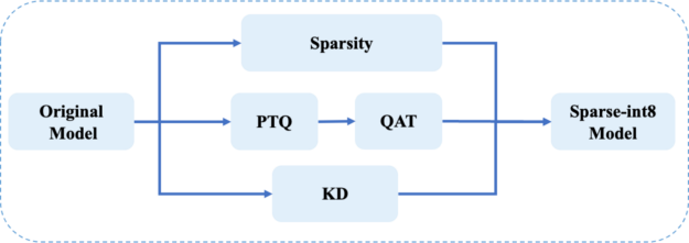
Sparse-QAT: Combine sparsity with quantization and distillation
To obtain lighter models, you can further combine sparsity with quantization and distillation in a method called sparse-QAT.
Quantization (PTQ and QAT)
The following equation formulates a general quantization procedure. For a float32 value x, use \(Q[x]\) to denote its quantized value with K-bit representation.
\(Q[x] = s \times round \bigl( clamp \left( \frac{x}{s},l_{min},l_{max} \right) \bigr)\)
In general, you first quantize the original parameters to a certain range and round them to integers. Then, you use the quantization scale to recover the original value. This motivates your first quantization method, calibration, also known as post-training quantization (PTQ).
In calibration, a critical thing is to set an appropriate quantization scale. If the scale is too large, it is less accurate for numbers within the range. On the contrary, if the scale is too small, it results in too many numbers outside the range of \(l_{min}\) to \(l_{max}\).
Therefore, to balance these two aspects, you first obtain the distribution of tensor values and then set the quantization scale to include 99.99% of the numbers. It has been proved in multiple works that this method is helpful in finding a good quantization scale during calibration.
However, although you have set a reasonable quantization scale for calibration, the accuracy still drops significantly for 8 bits. You then introduce quantization-aware training (QAT) to further improve the accuracy after calibration. The idea of QAT is to train a model with simulation quantization.
In the forward pass, you quantize the weights to int8 and dequantize them to float in the node to simulate quantization. In the backward pass, the gradients are used to update the model weights, which is called straight-through estimation (STE). The key idea is the following equation:
\(\frac{\partial f}{\partial x} = \frac{\partial f }{\partial Q[x] }\)
Gradients of values in the threshold ranges are passed directly in the backward pass, and gradients of values outside the threshold ranges are clipped to 0.
Knowledge distillation
In addition to the previous methods, we introduced knowledge distillation (KD) to further ensure the accuracy of the sparse-QAT model. Take the original model as the teacher and the quantized sparse model as the student.
During the fine-tuning process, we adopted mini-distillation, which is a layer-wise distillation. With MiniLM, you only have to use the self-attention output of the last transformer layer to do the distillation. You can even achieve higher accuracy than the teacher model after Sparse-QAT. For more information, see MiniLM: Deep Self-Attention Distillation for Task-Agnostic Compression of Pre-Trained Transformers.
Pipeline of Sparse-QAT
Figure 5 shows the pipeline of Sparse-QAT. You use sparsity, quantization, and KD together to get the final sparse-int8 model. There are three passes:
- Sparsity pass: Apply progressive sparsity to get a sparse tensor.
- Quantization pass: Use PTQ and QAT to get an int8 tensor.
- Knowledge distillation pass: Use MiniLM to guarantee the accuracy of the final sparse-int8 model.
Inference with NVIDIA Ampere architecture sparsity
After the sparse model is trained, you can use TensorRT and cuSPARSELt to accelerate the inference with NVIDIA Ampere architecture structured sparsity.
Inference with NVIDIA TensorRT
NVIDIA TensorRT supports sparse convolution as of version 8.0. GEMMs should be replaced with 1×1 convolutions to use the sparsity inference. Enabling sparsity in TensorRT is easy. Before importing into TensorRT, the weights of the model should have 2:4 sparsity. If trtexec is used to build the engine, set the –sparsity=enable flag. If you are writing codes or scripts to build the engine, set the build config as follows:
For C++: config->setFlag(BuilderFlag::kSPARSE_WEIGHTS)
For Python: config.set_flag(trt.BuilderFlag.SPARSE_WEIGHTS)
Use NVIDIA cuSPARSELt to enhance TensorRT
For some use cases, the input sizes may vary and TensorRT may not provide the best performance. You can use NVIDIA cuSPARSELt to further accelerate these cases.
The solution is to write TensoRT plug-ins with cuSPARSELt. Initialize multiple descriptors and plans of cuSPARSELt sparse GEMM for different input sizes and choose an appropriate plan for each input.
Assuming that you implement the SpmmPluginDynamic plug-in, it inherits from nvinfer1::IPluginV2DynamicExt and you use a private struct to store the plans.
 struct cusparseLtContext {
    cusparseLtHandle_t handle;
    std::vector<cusparseLtMatmulPlan_t> plans;
    std::vector<cusparseLtMatDescriptor_t> matAs, matBs, matCs;
    std::vector<cusparseLtMatmulDescriptor_t> matmuls;
    std::vector<cusparseLtMatmulAlgSelection_t> alg_sels;
}
A TensorRT plug-in should implement the configurePlugin method, which sets up the plug-in according to the input and output types and sizes. You initialize the cuSPARSELt-related structures in this method.
There is a constraint that the input size of cuSPARSELt should be a multiple of 4, 8, or 16 depending on the data type. For this post, we set it to a multiple of 16. For more information about the constraints, see cusparseLtDenseDescriptorInit.
for (int i = 0; i < size_num; ++i) {
  m = 16 * (i + 1);
  int alignment = 16;
  CHECK_CUSPARSE(cusparseLtStructuredDescriptorInit(
      &handle, &matBs[i], n, k, k, alignment, type, CUSPARSE_ORDER_ROW,
      CUSPARSELT_SPARSITY_50_PERCENT))
  CHECK_CUSPARSE(cusparseLtDenseDescriptorInit(
      &handle, &matAs[i], m, k, k, alignment, type, CUSPARSE_ORDER_ROW))
  CHECK_CUSPARSE(cusparseLtDenseDescriptorInit(
      &handle, &matCs[i], m, n, n, alignment, type, CUSPARSE_ORDER_ROW))
  CHECK_CUSPARSE(cusparseLtMatmulDescriptorInit(
      &handle, &matmuls[i], CUSPARSE_OPERATION_NON_TRANSPOSE,
      CUSPARSE_OPERATION_TRANSPOSE, &matAs[i], &matBs[i], &matCs[i], &matCs[i], compute_type))
  CHECK_CUSPARSE(cusparseLtMatmulAlgSelectionInit(
      &handle, &alg_sels[i], &matmuls[i], CUSPARSELT_MATMUL_ALG_DEFAULT))
  int split_k = 1;
  CHECK_CUSPARSE(cusparseLtMatmulAlgSetAttribute(
      &handle, &alg_sels[i], CUSPARSELT_MATMUL_SPLIT_K, &split_k, sizeof(split_k)))
  int alg_id = 0;
  CHECK_CUSPARSE(cusparseLtMatmulAlgSetAttribute(
      &handle, &alg_sels[i], CUSPARSELT_MATMUL_ALG_CONFIG_ID, &alg_id, sizeof(alg_id)))
  size_t ws{0};
  CHECK_CUSPARSE(cusparseLtMatmulPlanInit(&handle, &plans[i], &matmuls[i], &alg_sels[i],
                                          ws))
  CHECK_CUSPARSE(
      cusparseLtMatmulGetWorkspace(&handle, &plans[i], &ws))
  workspace_size = std::max(workspace_size, ws);
}
In the enqueue function, you can select the proper plan to do the matmul operation:
int m = inputDesc->dims.d[0];
int idx = (m + 15) / 16 - 1;
float alpha = 1.0f;
float beta = 0.0f;
auto input = static_cast<const float*>(inputs[0]);
auto output = static_cast<float*>(outputs[0]);
cusparseStatus_t status = cusparseLtMatmul(
    &handle, &plans[idx], &alpha, input,
    weight_compressed, &beta, output, output, workSpace, &stream, 1);
Some applications in search engines
In this section, we show four applications that take advantage of sparsity in search engines:
- Search relevance prediction aims to evaluate the relevance between the input text and the videos in the database.
- Query performance prediction is used for the document recall delivery strategy.
- A recall task for recalling the most relevant texts.
- The text-to-image task automatically generates corresponding pictures according to the input prompt.
Search relevance cases
The results of these cases are evaluated with positive negative rate (PNR) or accuracy (Acc).
In relevance case 1, we ran Sparse-QAT and obtained a sparse-int8 model with higher PNR than the online int8 model in two important evaluation indices.
| Model | Evaluation Index A | Evaluation Index B |
| float32 | 4.0138 | 3.1384 |
| int8 (online) | 3.9454 | 2.9120 |
| Sparse-int8 | 4.0406 | 2.9591 |
In relevance case 2, the sparse-int8 model can achieve comparable Acc scores to the float32 model with a 1.4x inference speedup compared to the dense-int8 model.
| Evaluation Index | |
| Bert_12L (float32) | 0.8015 |
| Bert_12L (sparse-int8) | 0.8010 |
Query performance prediction cases
In this section, we show four cases of query performance prediction (QPP) that are evaluated with normalized discounted cumulative gain (NDCG). As shown in Table 3, these sparse-fp16 models can achieve even higher accuracy than the original float32 models, with a four-fold speedup in inference and negligible impact on the NDCG.
| Case A | Case B | Case C | Case D | |
| NDCG (float32 model) | 39723 | 39858 | 39878 | 32471 |
| NDCG (sparse-float16) | 39744 | 39927 | 39909 | 32494 |
| Relative inference time (float32) | 1 | 1 | 1 | 1 |
| Relative inference time (sparse-float16) | 0.25 | 0.25 | 0.25 | 0.25 |
| Inference speedup | 4x | 4x | 4x | 4x |
Query-doc case
Table 4 shows the result of a query-doc case in the search engine. With the proposed sparse-QAT pipeline, the sparse-int8 models can achieve 1.4x inference speedup with negligible accuracy loss compared with the dense-int8 model.
| Acc | f1_345 | recall_345 | |
| FP32 model | 0.7839 | 0.8627 | 0.8312 |
| Sparse-int8 model | 0.7814 | 0.8622 | 0.8416 |
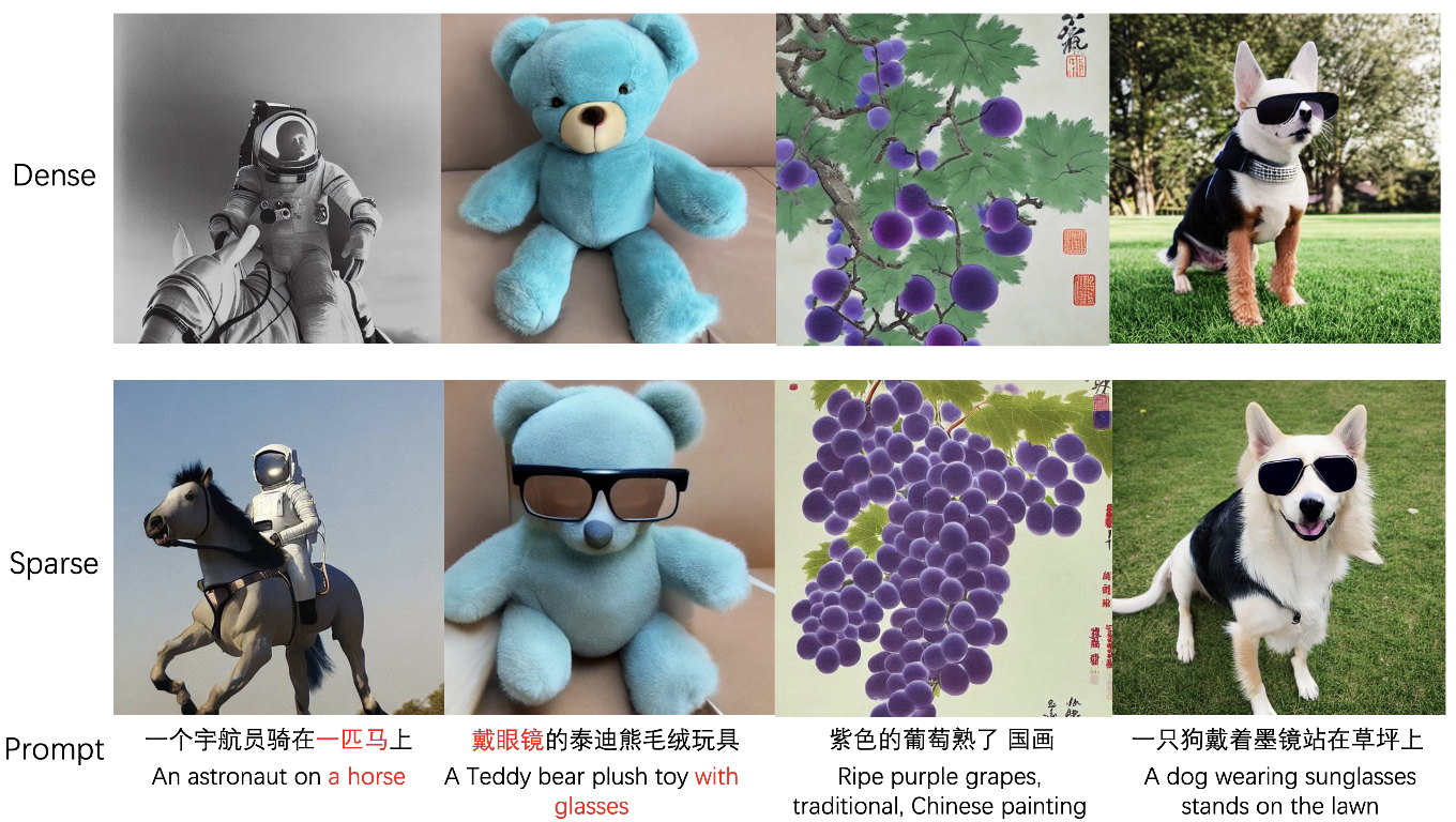
Text-to-image cases
Figure 6 shows the results of text-to-image models. The top four images are the output of the dense float32 model, and the bottom four images are the output of the sparse float16 model.
From the results, you can see that, given the same prompt, the sparse model can produce comparable results with the ones from the dense model. Some of the results are more reasonable as the model pruning and extra progressive sparse fine-tuning make the model learn more from the data.
Summary
The structured sparsity feature in the NVIDIA Ampere architecture can accelerate many deep learning workloads, and it is easy to use with TensorRT and cuSPARSELt.
For more information, see the Structured Sparsity in the NVIDIA Ampere Architecture and its Applications in Tencent WeChat Search GTC session. Download the latest TensorRT and cuSPARSELt versions.
