The training stage of deep learning (DL) models consists of learning numerous dense floating-point weight matrices, which results in a massive amount of floating-point computations during inference. Research has shown that many of those computations can be skipped by forcing some weights to be zero, with little impact on the final accuracy.
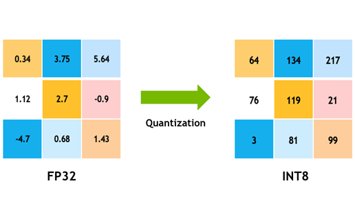
In parallel to that, previous posts have shown that lower precision, such as INT8, is often sufficient to obtain similar accuracies to FP32 during inference. Sparsity and quantization are popular optimization techniques used to tackle these points, improving inference time and reducing memory footprint.
Quantization support has been available in NVIDIA TensorRT for a while (as of the 2.1 release), and support for sparsity was more recently built into NVIDIA Ampere architecture Tensor Cores and introduced in TensorRT 8.0.
This post is a step-by-step guide on how to accelerate DL models with TensorRT using sparsity and quantization techniques. Although each of these optimizations has been individually discussed, there’s still a need to demonstrate the end-to-end workflow from training to deployment with TensorRT, considering both optimizations.
In this post, we aim to bridge that gap and to help you understand what the sparsity-quantization training workflow looks like, advise on best practices for sparsity with regards to TensorRT acceleration, and present an end-to-end case study with ResNet-34.
Structured sparsity
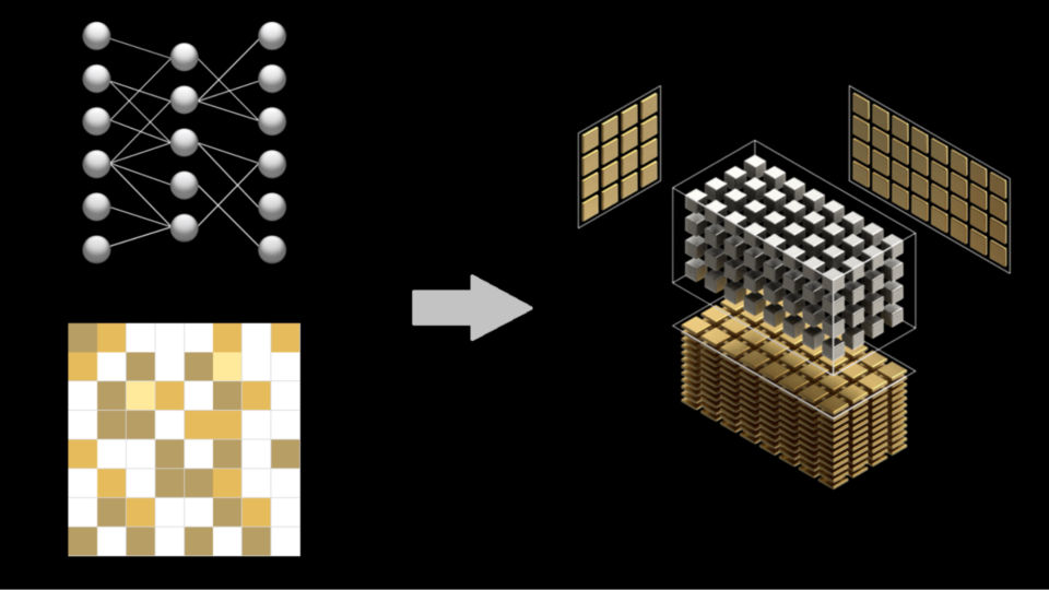
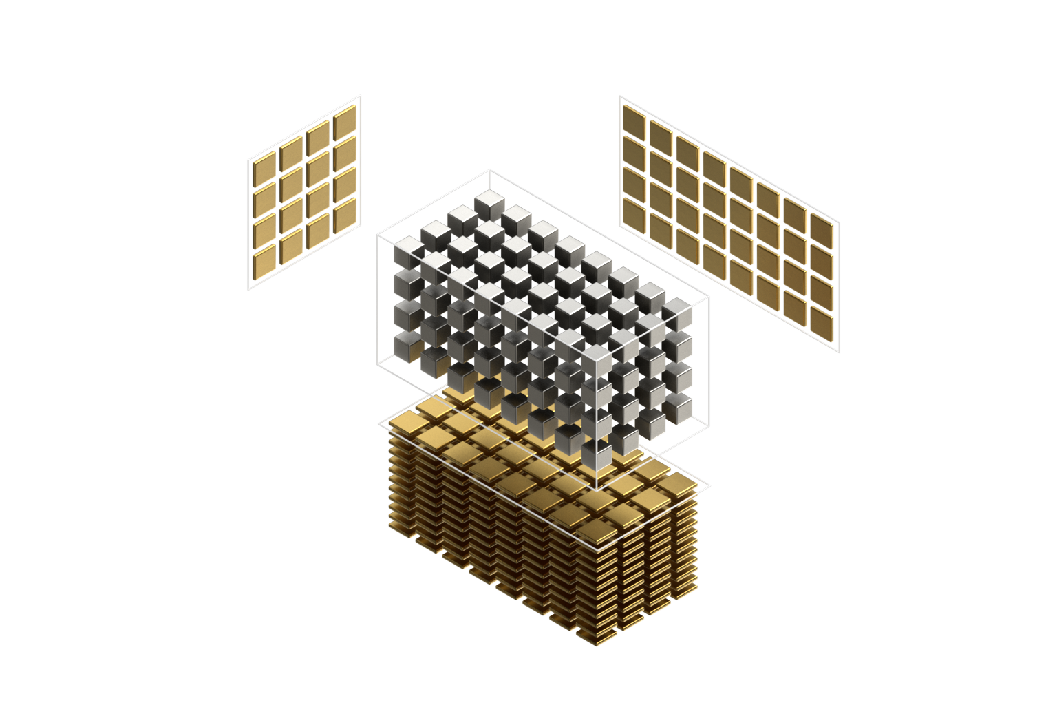
NVIDIA Sparse Tensor Cores use a 2:4 pattern, meaning that two out of each contiguous block of four values must be zero. In other words, we follow a 50% fine-grained structured sparsity recipe, with no computations being done on zero-values due to the available support directly on the Tensor Cores. This results in more workload being computed in the same amount of time. In this post, we refer to this process as pruning.
For more information, see Accelerating Inference with Sparsity Using the NVIDIA Ampere Architecture and NVIDIA TensorRT.
Quantization
Quantization refers to the process of mapping continuous infinite values to a finite set of discrete values (for example, FP32 to INT8). There are two main quantization techniques discussed in this post:
- Post-training quantization (PTQ): Uses an implicit quantization workflow. In implicitly quantized networks, each quantized tensor has an associated scale that is used to implicitly quantize and dequantize values through calibration. TensorRT then checks in which precision that layer runs faster and executes it accordingly.
- Quantization-aware training (QAT): Uses an explicit quantization workflow. Explicitly quantized networks make use of quantize and dequantize (Q/DQ) nodes to explicitly indicate which layers must be quantized. This means that you have more control over which layers are running in INT8. For more information, see Q/DQ Layer-Placement Recommendations.
For more information about quantization basics, a comparison between PTQ and QAT quantization techniques, insights on when to choose which, and quantization in TensorRT, see Achieving FP32 Accuracy for INT8 Inference Using Quantization Aware Training with NVIDIA TensorRT.
Workflow for deploying sparse-quantized models in TensorRT
The workflow for deploying sparse-quantized models in TensorRT, considering PyTorch as the DL framework, has the following steps:
- Sparsifying and fine-tuning a pretrained dense model in PyTorch.
- Quantizing the sparsified model through the PTQ or QAT workflow.
- Deploying the obtained sparse INT8 engine in TensorRT.
Figure 1 shows all three steps. One distinction in step 2 is that Q/DQ nodes are present in the ONNX graph generated through QAT but absent in the ONNX graph generated through PTQ. For more information, see Working with INT8.
Given that, here’s the full workflow for QAT:
- Sparsifying and fine-tuning a pretrained dense model in PyTorch.
- Quantizing, calibrating, and fine-tuning the sparsified model in PyTorch.
- Exporting the PyTorch model to ONNX.
- Generating a TensorRT engine through ONNX.
- Deploying the obtained Sparse INT8 engine in TensorRT.
On the other hand, here’s the full workflow for PTQ:
- Sparsifying and fine-tuning a pretrained dense model in PyTorch.
- Exporting the PyTorch model to ONNX.
- Calibrating and quantizing the sparsified ONNX model through the TensorRT builder, generating a TensorRT engine.
- Deploying the obtained sparse INT8 engine in TensorRT.
Case study: ResNet-34
This section demonstrates a case study of the Sparsity-Quantization workflow with ResNet-34. For more information, see the full code example on the /SparsityINT8 GitHub repo.
Requirements
Here’s the basic configuration required to follow this case study:
- Python 3.8
- PyTorch 1.11 (also tested with 2.0.0)
- PyTorch vision
- apex sparsity toolkit
- pytorch-quantization toolkit
- TensorRT 8.6
- Polygraphy
- ONNX opset>=13
- NVIDIA Ampere architecture GPU for Tensor Core support
This case study requires the ImageNet 2012 dataset for image classification. For more information about downloading the dataset and converting it to the required format, see the readme on the GitHub repo.
This dataset is needed for sparsity training, sparse-QAT model fine-tuning, and sparse-PTQ model calibration. It is also used to evaluate the models.
Step 1: Sparsify and fine-tune from the dense model
Load the pretrained dense model and augment the model and the optimizer for sparsity training. For more information, see the NVIDIA/apex/tree/master/apex/contrib/sparsity folder.
import copy
from torchvision import models
from apex.contrib.sparsity import ASP

# Load dense model
model_dense = models.__dict__["resnet34"](pretrained=True)

# Initialize sparsity mode before starting sparse training
model_sparse = copy.deepcopy(model_dense)
ASP.prune_trained_model(model_sparse, optimizer)

# Re-train model
for e in range(0, epoch):
    for i, (image, target) in enumerate(data_loader):
        image, target = image.to(device), target.to(device)
        output = model_sparse(image)
        loss = criterion(output, target)
        optimizer.zero_grad()
        loss.backward()
        optimizer.step()

# Save model
torch.save(model_sparse.state_dict(), "sparse_finetuned.pth")
Step 2: Quantize the PyTorch model
There are two quantization methods that you can choose for this step: PTQ or QAT.
PTQ through TensorRT calibration
This option exports a PyTorch model to ONNX and calibrates it through the TensorRT Python API. This generates a calibration cache and a TensorRT engine that is ready for deployment.
Export the sparse PyTorch model to ONNX:
dummy_input = torch.randn(batch_size, 3, 224, 224, device="cuda")
torch.onnx.export(model_sparse, dummy_input, "sparse_finetuned.onnx", opset_version=13, do_constant_folding=True)
Calibrate the ONNX model, exported in the previous step, with a calibration dataset. The following code example assumes an ONNX model with static input shape and batch size.
from infer_engine import infer
from polygraphy.backend.trt import Calibrator, CreateConfig, EngineFromNetwork, NetworkFromOnnxPath, TrtRunner, SaveEngine
from polygraphy.logger import G_LOGGER


# Data loader argument to `Calibrator`
def calib_data(val_batches, input_name):
    for iteration, (images, labels) in enumerate(val_batches):
        yield {input_name: images.numpy()}

# Set path to ONNX model
onnx_path = "sparse_finetuned.onnx"

# Set calibrator
calibration_cache_path = onnx_path.replace(".onnx", "_calibration.cache")
calibrator = Calibrator(
    data_loader=calib_data(data_loader_calib, args.onnx_input_name),
    cache=calibration_cache_path
)

# Build engine from ONNX model by enabling INT8 and sparsity weights, and providing the calibrator
build_engine = EngineFromNetwork(
    NetworkFromOnnxPath(onnx_path),
    config=CreateConfig(
        int8=True,
        calibrator=calibrator,
        sparse_weights=True
    )
)

# Trigger engine saving
engine_path = onnx_path.replace(".onnx", ".engine")
build_engine = SaveEngine(build_engine, path=engine_path)

# Calibrate engine (activated by the runner)
with G_LOGGER.verbosity(G_LOGGER.VERBOSE), TrtRunner(build_engine) as runner:
    print("Calibrated engine!")

    # Infer PTQ engine and evaluate its accuracy
    log_file = engine_path.split("/")[-1].replace(".engine", "_accuracy.txt")
    infer(
        engine_path,
        data_loader_test,
        batch_size=args.batch_size,
        log_file=log_file
    )
QAT through the pytorch-quantization toolkit
This option uses the pytorch-quantization toolkit to add Q/DQ nodes in the Sparse PyTorch model, calibrates it, and fine-tunes it for a few epochs. The fine-tuned model is then exported to ONNX and converted to a TensorRT engine for deployment.
To ensure that the already-calculated sparse floating-point weights won’t be overwritten, ensuring that the QAT weights will also be structured as sparse, you must again prepare the model for pruning.
Initialize the QAT model and optimizer for pruning before loading the fine-tuned sparse weights. Sparse mask re-computations must also be disabled as they were already computed in Step 1. This requires a custom function that is a slight modification of the APEX toolkit’s prune_trained_model function. The modifications are highlighted in the code example:
from apex.contrib.sparsity import ASP

def prune_trained_model_custom(model, optimizer, compute_sparse_masks=False):
    asp = ASP()
    asp.init_model_for_pruning(model, mask_calculator="m4n2_1d", verbosity=2, whitelist=[torch.nn.Linear, torch.nn.Conv2d], allow_recompute_mask=False)
    asp.init_optimizer_for_pruning(optimizer)
    if compute_sparse_masks:
        asp.compute_sparse_masks()
For optimal Q/DQ node placement, you must modify the model’s definition to quantize residual branches, as shown in the pytorch-quantization toolkit example. For example, for ResNet, the modification needed to add Q/DQ nodes in the residual branch are highlighted as follows:
from pytorch_quantization import nn as quant_nn

class BasicBlock(nn.Module):

   def __init__(self, ..., quantize: bool = False) -> None:
       super().__init__()
       ...
       if self._quantize:
            self.residual_quantizer = quant_nn.TensorQuantizer(quant_nn.QuantConv2d.default_quant_desc_input)

   def forward(self, x: Tensor) -> Tensor:
       identity = x
       ...
       if self._quantize:
           out += self.residual_quantizer(identity)
       else:
           out += identity
       out = self.relu(out)
       return out
The same modification must be repeated for the Bottleneck class and the quantize bool parameter must be propagated through the ResNet, _resnet, and resnet34 functions. After those modifications are done, instantiate the model with quantize=True. For more information, see line 734 in resnet.py.
The first step of quantizing a sparse model through QAT is to enable quantization and pruning in the model. The second step is to load the fine-tuned sparse checkpoint, calibrate it, and then finally fine-tune that model for some epochs. For more information about the collect_stats and compute_amax functions, see the calibrate_quant_resnet50.ipynb notebook.
# Add Q/DQ nodes to the dense model
from pytorch_quantization import quant_modules
quant_modules.initialize()
model_qat = models.__dict__["resnet34"](pretrained=True, quantize=True)

# Initialize sparsity mode before starting Sparse-QAT fine-tuning
prune_trained_model_custom(model_qat, optimizer, compute_sparse_masks=False)

# Load Sparse weights
load_dict = torch.load("sparse_finetuned.pth")
model_qat.load_state_dict(load_dict["model_state_dict"])

# Calibrate model
collect_stats(model_qat, data_loader_calib, num_batches=len(data_loader_calib))
compute_amax(model_qat, method="entropy”)

# Fine-tune model
for e in range(0, epoch):
    for i, (image, target) in enumerate(data_loader):
        image, target = image.to(device), target.to(device)
        output = model_qat(image)
        ...

# Save model
torch.save(model_qat.state_dict(), "quant_finetuned.pth")
To prepare the TensorRT engine for deployment, you must export the sparse-quantized PyTorch model to ONNX. TensorRT expects QAT ONNX models to indicate which layers should be quantized through a set of QuantizeLinear and DequantizeLinear ONNX ops. This requirement is fulfilled by enabling fake quantization when exporting a quantized PyTorch model to ONNX.
from pytorch_quantization import nn as quant_nn
quant_nn.TensorQuantizer.use_fb_fake_quant = True
dummy_input = torch.randn(batch_size, 3, 224, 224, device="cuda")
torch.onnx.export(model_qat, dummy_input, "quant_finetuned.onnx", opset_version=13, do_constant_folding=True)
Finally, build the TensorRT engine:
$ trtexec --onnx=quant_finetuned.onnx --int8 --sparsity=enable --saveEngine=quant_finetuned.engine --skipInference
Step 3: Deploy the TensorRT engine
$ trtexec --loadEngine=quant_finetuned.engine -v
Results
Here are the performance measurements, in terms of classification accuracy and runtime, for ResNet-34 dense-quantized and sparse-quantized models on an NVIDIA A40 GPU with TensorRT 8.6-GA (8.6.1.6). To reproduce these results, follow the workflow described in the previous section.
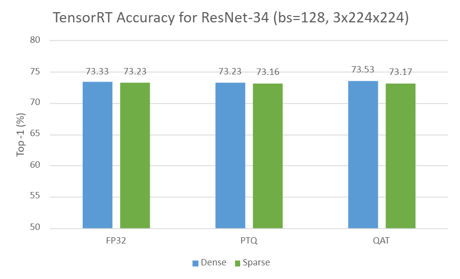
Figure 2 shows the dense accuracy compared to sparse accuracy in TensorRT for ResNet-34 in three settings:
- Dense vs. sparse in FP32
- Dense-PTQ vs. sparse-PTQ in INT8
- Dense-QAT vs. sparse-QAT in INT8
As you can see, the sparse variants can mostly preserve accuracy compared to their dense equivalents for all settings.
Input resolution of 3x224x224, using TensorRT 8.6-GA.
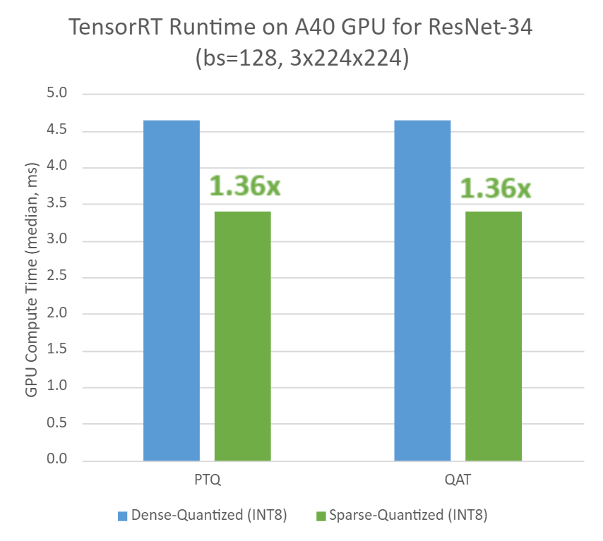
In regard to runtime performance, Figure 3 shows a ~1.4x speedup for sparse-quantized models over dense-quantized for both PTQ and QAT workflows.
Batch sizes and input resolutions
A large workload gives sparse kernels more of an opportunity to shine. In this section, we evaluate how different batch sizes (bs) and input resolutions affect speedups between dense and sparse models running in INT8 precision.
Figure 4 shows a speedup improvement between dense-quantized and sparse-quantized settings in ResNet-34 as batch size increases for both PTQ and QAT workflows.
- Speedup for the PTQ workflow ranges from 1.21x for bs=1 up to 1.40x for bs=2048.
- Speedups for the QAT workflow are in the same ballpark, ranging from 1.20x for bs=1 up to 1.42x for bs=2048.
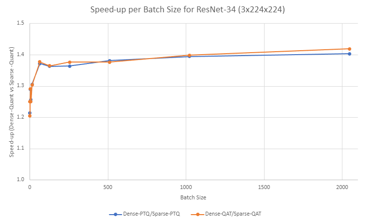
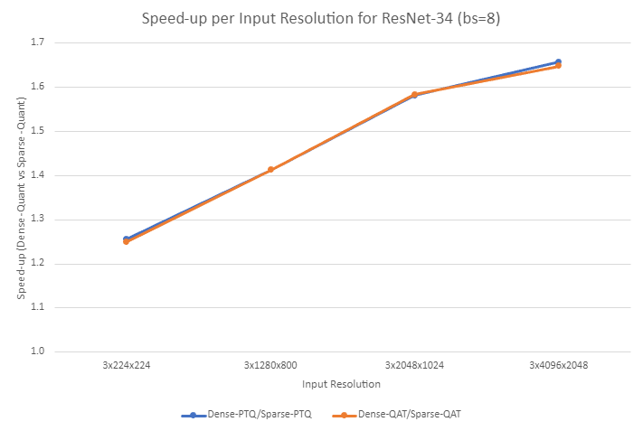
Figure 5 shows a speedup improvement between dense-quantized and sparse-quantized settings in ResNet-34 as input resolution increases for both PTQ and QAT workflows. Speedups for the PTQ and QAT workflows range from 1.26x and 1.25x for input resolution of 3x224x224, up to 1.66x and 1.65x for input resolution of 3x4096x2048, respectively.
Here are some additional best practices that we observed during our experiments:
- Output channels in a multiple of 32 are friendly to leverage TensorCore or IMMA for INT8. For more information, see Deep Learning Performance Guide.
- High output channels (typically >128) help better pick up sparse kernels due to the large workload.
Conclusion
In this post, we demonstrated that significant latency reduction can be achieved with minimal impact on accuracy through a sparse INT8-based training workflow and TensorRT deployment strategies. We provided a thorough step-by-step guide with ResNet-34 as a use case, followed up by a discussion on the observed performance with respect to accuracy and latency.
Experimental results showed that accuracy was mostly maintained when comparing dense and sparse models, while runtime improved to up to ~1.7x for the highest explored workload (input resolution 3x4096x2048, bs=8). Finally, we shared some best practices for sparsity that we observed during our experiments.
For more information about sparsity, see the following related resources:
- Accelerating Inference with Sparsity Using the NVIDIA Ampere Architecture and NVIDIA TensorRT
- Making the Most of Structured Sparsity in the NVIDIA Ampere Architecture (GTC session)
- Accelerating Sparsity in the NVIDIA Ampere Architecture (GTC session)
- Accelerating Sparse Deep Neural Networks (whitepaper)
For more information about quantization, see the following related resources:
- Achieving FP32 Accuracy for INT8 Inference Using Quantization Aware Training with NVIDIA TensorRT
- Accelerating Quantized Networks with the NVIDIA QAT Toolkit for TensorFlow and NVIDIA TensorRT
- Toward INT8 Inference: An End-to-End Workflow for Deploying Quantization-Aware Trained Networks Using TensorRT (GTC session)
- Integer Quantization for Deep Learning Inference: Principles and Empirical Evaluation (whitepaper)


