
This series on the RAPIDS ecosystem explores the various aspects that enable you to solve extract, transform, load (ETL) problems, build machine learning (ML) and deep learning (DL) models, explore expansive graphs, process signal and system logs, or use the SQL language through BlazingSQL to process data. For part 1, see Pandas DataFrame Tutorial: A Beginner’s Guide to GPU Accelerated DataFrames in Python.

As the data science field has grown immensely over the last decade, the appetite among data scientists for compute power to handle the data volume has been steadily increasing as well. Around 15 to 20 years ago, the most common choices to process data were limited to SAS and SQL-based solutions. These included SQL Server, Teradata, PostGRE, or MySQL; R if you were heavy on statistical methods; or Python if you wanted the versatility of a general-purpose language at the expense of some statistical features.
Over the years, many solutions were introduced to handle the ever-growing stream of data. Hadoop was released in 2006 and it gained popularity only to be dethroned by Apache Spark as a go-to tool for processing data in a distributed way.
However, using Spark brought new challenges. For people familiar with pandas and other tools from the PyData ecosystem, it meant learning a new API. For businesses, it meant rewriting their code base to run in a distributed environment of Spark.
Dask bridged this gap by adding the distributed support to already existing PyData objects like pandas DataFrames or NumPy arrays and made it that much easier to harness the full power of the CPU or of a distributed cluster without extensive code rewrites. However, processing large amounts of data in an interactive manner was (and still is) beyond reach for reasonably sized and priced CPU clusters.
RAPIDS changed that landscape in late 2018. Paired with Dask, RAPIDS taps into the enormous parallelism of NVIDIA GPUs to process the data. However, unlike Apache Spark, it does not introduce a new API but provides a familiar programming interface of tools found in the PyData ecosystem, like pandas, scikit-learn, NetworkX, and more.

The first post in this series was a python pandas tutorial where we introduced RAPIDS cuDF, the RAPIDS CUDA DataFrame library for processing large amounts of data on an NVIDIA GPU.
In this tutorial, we discuss how cuDF is almost an in-place replacement for pandas. To aid with this, we also published a downloadable cuDF cheat sheet.
Popular interface
If you work with data using Pytho,n you have quite likely been using pandas or NumPy, as pandas builds on top of NumPy. It is hard to overstate the great value that these two libraries provide to the PyData ecosystem. pandas has been the basis for almost all data manipulation and massaging. It has been seen in countless notebooks published on GitHub, Kaggle, Towards Data Science, and more. Chances are, if you are looking for a solution to your data problem using Python, you are likely to be shown examples that employ pandas.
RAPIDS cuDF, almost entirely, replicates the same API and functionality. While not 100% feature-equivalent with pandas, the team at NVIDIA and external contributors work continually on bridging the feature-parity gap.
Moving between these two frameworks is extremely easy. Consider a simple pandas script that reads the data, calculates descriptive statistics for a DataFrame, and then performs a simple data aggregation.
# pandas
import pandas as pd
df = pd.read_csv('df.csv')
(
   df
    .groupby(by='category')
    .agg({'num': 'sum', 'char': 'count'})
    .reset_index()
)
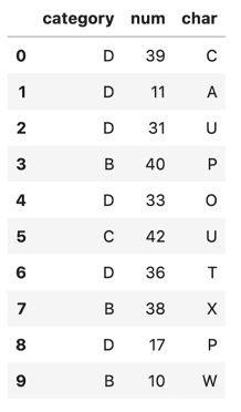
Peek inside the df DataFrame,
df.head(10)You get the output in Figure 1.
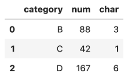
The aggregation step accurately provides the final result:
With RAPIDS, all you have to do to use this code to run on a GPU and enjoy the interactive querying of data is to change the import statement.
# cudf
import cudf
df = cudf.read_csv('../results/pandas_df_with_index.csv')
(
    df
    .groupby(by='category')
    .agg({'num': 'sum', 'char': 'count'})
    .reset_index()
)
You literally changed one import statement and are now running on a GPU!
On a small dataset like this, it takes milliseconds to run things with pandas and everybody is happy. How about processing a DataFrame with 100M records? In this example for a larger data set, you use CuPy to speed things up a little.
import cupy as cp
choices = range(6)
probs = cp.random.rand(6)
s = sum(probs)
probs = [e / s for e in probs]
n = int(100e6)  ## 100M
selected = cp.random.choice(choices, n, p=probs)
nums = cp.random.randint(10, 1000, n)
chars = cp.random.randint(65,80, n)
The NumPy equivalent of that code would be as follows:
import numpy as np
choices = range(6)
probs = np.random.rand(6)
s = sum(probs)
probs = [e / s for e in probs]
n = int(100e6)  ## 100M
selected = np.random.choice(choices, n, p=probs)
nums = np.random.randint(10, 1000, n)
chars = np.random.randint(65,80, n)
nNotice any differences? Yes, only the import statement! And time: the CuPy version runs in about 1.27 seconds on an NVIDIA Titan RTX while the NumPy version on an i5 CPU takes roughly 3.33 seconds.
You can now use the CuPy or NumPy arrays to create cuDF or pandas DataFrames. Here’s the example for a cuDF DataFrame:
import cudf
df = cudf.DataFrame({
    'category': selected
    , 'num': nums
    , 'char': chars
})
df['category'] = df['category'].astype('category')
Here’s the example for creating a pandas DataFrame:
import pandas
df = pandas.DataFrame({
    'category': selected
    , 'num': nums
    , 'char': chars
})
df['category'] = pandas_df['category'].astype('category')
The time needed to create these examples are negligible, as both cuDF and pandas simply retrieve pointers to the created CuPy and NumPy arrays. Still, you have so far only changed the import statements.
The aggregation code is the same as what was used earlier, with no changes between cuDF and pandas DataFrames. Neat! However, the execution times are quite different. It took, on average, 68.9 ms +/- 3.8 ms (7 runs, 10 loops each) for the cuDF code to finish while the pandas code took, on average, 1.37s +/- 1.25 ms (7 runs, 10 loops each). This equates to a roughly 20x speedup! And did I mention no code changes?!
Custom kernels
In some instances, minor code adaptations when moving from pandas to cuDF are required when it comes to custom functions used to transform data.
RAPIDS cuDF, being a GPU library built on top of NVIDIA CUDA, cannot take regular Python code and simply run it on a GPU. cuDF uses Numba to convert and compile the Python code into a CUDA kernel. Scared already? Don’t be! No direct knowledge of CUDA is necessary to run your custom transform functions using cuDF.
Consider the following example in pandas that calculates a regression line given two features:
# pandas
def pandas_regression(a, b, A_coeff, B_coeff, constant):
    return A_coeff * a + B_coeff * b + constant

<hr>
pandas_df['output'] = pandas_df.apply(
    lambda row: pandas_regression(
        row['num']
        , row['float']
        , A_coeff=0.21
        , B_coeff=-2.82
        , constant=3.43
    ), axis=1)
Pretty straightforward. To achieve the same outcome in cuDF, it is a little bit different but still readable and easily convertible.
# cudf
def cudf_regression(a, b, output, A_coeff, B_coeff, constant):
    for i, (aa, bb) in enumerate(zip(a,b)):
        output[i] = A_coeff * aa + B_coeff * bb + constant

<hr>
cudf_df.apply_rows(
    cudf_regression
    , incols = {'num': 'a', 'float': 'b'}
    , outcols = {'output': np.float64}
    , kwargs = {'A_coeff': 0.21, 'B_coeff': -2.82, 'constant': 3.43}
)
Numba takes the cudf_regression function and compiles it to the CUDA kernel. The apply_rows call is equivalent to the apply call in pandas with the axis parameter set to 1, that is, iterate over rows rather than columns. In cuDF, you must also specify the data type of the output column so that Numba can provide the correct return type signature to the CUDA kernel.
Despite these differences, though, the code is still a close equivalent to the pandas version. It differs mostly in the API call: the regression line is calculated in almost the same way. Here’s the Numba version:
return A_coeff * a + B_coeff * b + constant
Here’s the pandas version:
output[i] = A_coeff * aa + B_coeff * bb + constantIf you use operations on strings, DateTimes, or categorical columns, see the cuDF4pandas cheat sheet.
Update 11/20/2023: RAPIDS cuDF now comes with a pandas accelerator mode that allows you to run existing pandas workflow on GPUs with up to 150x speed-up requiring zero code change while maintaining compatibility with third-party libraries. The code in this blog still functions as expected, but we recommend using the pandas accelerator mode for seamless experience. Learn more about the new release in this TechBlog post.
