Parallel reduction is a common building block for many parallel algorithms. A presentation from 2007 by Mark Harris provided a detailed strategy for implementing parallel reductions on GPUs, but this 6-year old document bears updating. In this post I will show you some features of the Kepler GPU architecture which make reductions even faster: the shuffle (SHFL) instruction and fast device memory atomic operations.
The source code for this post is available on Github.
Shuffle On Down
Efficient parallel reductions exchange data between threads within the same thread block. On earlier hardware this meant using shared memory, which involves writing data to shared memory, synchronizing, and then reading the data back from shared memory. Kepler’s shuffle instruction (SHFL) enables a thread to directly read a register from another thread in the same warp (32 threads). This allows threads in a warp to collectively exchange or broadcast data. As described in the post “Do the Kepler Shuffle”, there are four shuffle intrinsics: __shfl(), __shfl_down(), __shfl_up(), and __shfl_xor(), but in this post we only use __shfl_down(), defined as follows: (You can find a complete description of the other shuffle functions in the CUDA C Programming Guide.)
int __shfl_down(int var, unsigned int delta, int width=warpSize);
__shfl_down() calculates a source lane ID by adding delta to the caller’s lane ID (the lane ID is a thread’s index within its warp, from 0 to 31). The value of var held by the resulting lane ID is returned: this has the effect of shifting var down the warp by delta lanes. If the source lane ID is out of range or the source thread has exited, the calling thread’s own var is returned. The ID number of the source lane will not wrap around the value of width and so the upper delta lanes will remain unchanged. Note that width must be one of (2, 4, 8, 16, 32). For brevity, the diagrams that follow show only 8 threads in a warp even though the warp size of all current CUDA GPUs is 32.
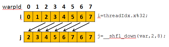
As an example, Figure 1 shows the effect of the following two lines of code, where we can see that values are shifted down by 2 threads.
int i = threadIdx.x % 32;
int j = __shfl_down(i, 2, 8);
There are three main advantages to using shuffle instead of shared memory:
- Shuffle replaces a multi-instruction shared memory sequence with a single instruction, increasing effective bandwidth and decreasing latency.
- Shuffle does not use any shared memory.
- Synchronization is within a warp and is implicit in the instruction, so there is no need to synchronize the whole thread block with
__syncthreads().
Note also that the Kepler implementation of shuffle instruction only supports 32-bit data types, but you can easily use multiple calls to shuffle larger data types. Here is a double-precision implementation of __shfl_down(). [Update June 2016: in recent versions of CUDA __shfl supports some larger types including double precision. The example is left here as a reference for other types that may not be supported].
__device__ inline
double __shfl_down(double var, unsigned int srcLane, int width=32) {
  int2 a = *reinterpret_cast<int2*>(&var);
  a.x = __shfl_down(a.x, srcLane, width);
  a.y = __shfl_down(a.y, srcLane, width);
  return *reinterpret_cast<double*>(&a);
}
Note also that threads may only read data from another thread which is actively participating in the __shfl() command. If the target thread is inactive, the retrieved value is undefined. Therefore, the code examples in this post assume that the block size is a multiple of the warp size (32). Note that the shuffle size can be reduced with the third parameters, but it must be a power of two, and the examples in this post are written for shuffles of 32 threads for highest efficiency.
Shuffle Warp Reduce
Now that we understand what shuffle is let’s look at how we can use it to reduce within a warp. Figure 2 shows how we can use shuffle down to build a reduction tree. Please note that I have only included the arrows for the threads that are contributing to the final reduction. In reality all threads will be shifting values even though they are not needed in the reduction.
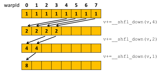
After executing the three reduction thread 0 has the total reduced value in its variable v. We’re now ready to write the following complete shfl-based warp reduction function.
__inline__ __device__
int warpReduceSum(int val) {
  for (int offset = warpSize/2; offset > 0; offset /= 2)
    val += __shfl_down(val, offset);
  return val;
}
Note, if all threads in the warp need the result, you can implement an “all reduce” within a warp using __shfl_xor() instead of __shfl_down(), like the following. Either version can be used in the block reduce of the next section.
__inline__ __device__
int warpAllReduceSum(int val) {
  for (int mask = warpSize/2; mask > 0; mask /= 2)
    val += __shfl_xor(val, mask);
  return val;
}
Block Reduce
Using the warpReduceSum function we can now easily build a reduction across the entire block. To do this we first reduce within warps. Then the first thread of each warp writes its partial sum to shared memory. Finally, after synchronizing, the first warp reads from shared memory and reduces again.
__inline__ __device__
int blockReduceSum(int val) {

  static __shared__ int shared[32]; // Shared mem for 32 partial sums
  int lane = threadIdx.x % warpSize;
  int wid = threadIdx.x / warpSize;

  val = warpReduceSum(val);     // Each warp performs partial reduction

  if (lane==0) shared[wid]=val; // Write reduced value to shared memory

  __syncthreads();              // Wait for all partial reductions

  //read from shared memory only if that warp existed
  val = (threadIdx.x < blockDim.x / warpSize) ? shared[lane] : 0;

  if (wid==0) val = warpReduceSum(val); //Final reduce within first warp

  return val;
}
As with warpReduceSum this function returns the reduced value on the first thread only. If all threads need the reduced value this could be quickly broadcast out by writing the reduce value to shared memory, calling __syncthreads, and reading the value in all threads.
Reducing Large Arrays
Now that we can reduce within a thread block, let’s look at how to reduce across a complete grid (many thread blocks). Reducing across blocks means global communication, which means synchronizing the grid, and that requires breaking our computation into two separate kernel launches. The first kernel generates and stores partial reduction results, and the second kernel reduces the partial results into a single total. We can actually do both steps with the following simple kernel code.
__global__ void deviceReduceKernel(int *in, int* out, int N) {
  int sum = 0;
  //reduce multiple elements per thread
  for (int i = blockIdx.x * blockDim.x + threadIdx.x;
       i < N;
       i += blockDim.x * gridDim.x) {
    sum += in[i];
  }
  sum = blockReduceSum(sum);
  if (threadIdx.x==0)
    out[blockIdx.x]=sum;
}
This kernel uses grid-stride loops (see the post “CUDA Pro Tip: Write Flexible Kernels with Grid Stride Loops”), which has two advantages: it allows us to reuse the kernel for both passes, and it computes per-thread sums in registers before calling blockReduceSum(). Doing the sum in registers significantly reduces the communication between threads for large array sizes. Note that the output array must have a size equal to or larger than the number of thread blocks in the grid because each block writes to a unique location within the array.
The code to launch the kernels on the host is straightforward.
void deviceReduce(int *in, int* out, int N) {
  int threads = 512;
  int blocks = min((N + threads - 1) / threads, 1024);

  deviceReduceKernel<<<blocks, threads>>>(in, out, N);
  deviceReduceKernel<<<1, 1024>>>(out, out, blocks);
}
Here you can see that the first pass reduces using 1024 blocks of 512 threads each, which is more than enough threads to saturate Kepler. We have chosen to restrict this phase to only 1024 blocks so that we only have 1024 partial results. In CUDA the maximum block size is 1024 threads. Since we have restricted the number of partial results to 1024 we can perform the second reduction phase of with a single block of 1024 threads.
In a previous CUDA pro-tip we discussed how to increase performance by using vector loads. We can apply the same technique to reduction, and while I won’t discuss that optimization in this post, you can find our vectorized solutions in the source on Github.
Atomic Power
Another Kepler architecture feature is fast device memory atomic operations, so let’s look at how we can use atomics to optimize reductions. The first way is to reduce across the warp using shuffle and then have the first thread of each warp atomically update the reduced value, as in the following code.
__global__ void deviceReduceWarpAtomicKernel(int *in, int* out, int N) {
  int sum = int(0);
  for(int i = blockIdx.x * blockDim.x + threadIdx.x;
      i < N;
      i += blockDim.x * gridDim.x) {
    sum += in[i];
  }
  sum = warpReduceSum(sum);
  if ((threadIdx.x & (warpSize - 1)) == 0)
    atomicAdd(out, sum);
}
Here we can see the kernel looks very similar to the deviceReduceKernel() above, but instead of assigning the partial reduction to the output array we atomically add the partial reduction directly to final reduction value in memory. This code is much simpler because it launches only a single kernel and it doesn’t use shared memory, a temporary global array, or any __syncthreads(). The disadvantage is that there could be a lot of atomic collisions when adding the partials. However, in applications where there are not many collisions this is a great approach. Another possibly significant disadvantage is that floating point reductions will not be bit-wise exact from run to run, because of the different order of additions (floating point arithmetic is not associative [PDF]).
Another way to use atomics would be to reduce the block and then immediately use atomicAdd().
__global__ void deviceReduceBlockAtomicKernel(int *in, int* out, int N) {
  int sum = int(0);
  for(int i = blockIdx.x * blockDim.x + threadIdx.x;
      i < N;
      i += blockDim.x * gridDim.x) {
    sum += in[i];
  }
  sum = blockReduceSum(sum);
  if (threadIdx.x == 0)
    atomicAdd(out, sum);
}
This approach requires fewer atomics than the warp atomic approach, executes only a single kernel, and does not require temporary memory, but it does use __syncthreads() and shared memory. This kernel could be useful when you want to avoid two kernel calls or extra allocation but have too much atomic pressure to use warpReduceSum() with atomics.
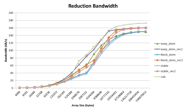
Figure 3 compares the performance of the three device reduction algorithms on a Tesla K20X GPU.
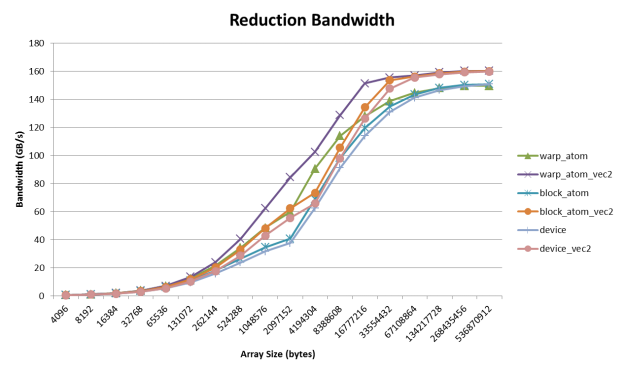
Here we can see that the warpReduceSum followed by atomics is the fastest. Thus if you are working on integral data or are able to tolerate changes in the order of operations you may want to consider using atomics. In addition we can see that vectorizing provides a significant boost in performance.
The CUB Library
Now that we have covered the low-level details of how to write efficient reductions let’s look at an easier way that you should consider using first: a library. CUB is a library of common building blocks for parallel algorithms including reductions that is tuned for multiple CUDA GPU architectures and automatically picks the best algorithm for the GPU you are running on and the data size and type you are processing. Figure 4 shows that the performance of CUB matches or exceeds our custom reduction code.
Interleaving Multiple Reductions
Before I end this post there is one last trick that I would like to leave you with. It is common to need to reduce multiple fields at the same time. A simple solution is to reduce one field at a time (for example by calling reduce multiple times). But this is not the most efficient method, so let’s look at the assembly for the warp reduction shown in Figure 5.
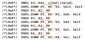
Here the arrows show dependencies; you can see that every instruction is dependent on the one before it, so there is no instruction-level parallelism (ILP) exposed. Perform multiple reductions at the same time by interleaving their instructions is more efficient because it increases ILP. The following code shows an example for an x, y, z triple.
__inline__ __device__
int3 warpReduceSumTriple(int3 val) {
  for (int offset = warpSize / 2; offset > 0; offset /= 2) {
    val.x += __shfl_down(val.x, offset);
    val.y += __shfl_down(val.y, offset);
    val.z += __shfl_down(val.z, offset);
  }
  return val;
}
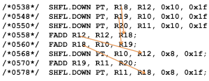
This leads to the SASS shown in Figure 6 (note that I have only shown the first few lines for brevity).
Here we can see we no longer have dependent instructions immediately following each other. Therefore more instructions are able to issue back-to-back without stalling, reducing the total exposed latency and thereby reducing the overall execution time.