
Quantitative finance libraries are software packages that consist of mathematical, statistical, and, more recently, machine learning models designed for use in quantitative investment contexts. They contain a wide range of functionalities, often proprietary, to support the valuation, risk management, construction, and optimization of investment portfolios.
Financial firms that develop such libraries must prioritize limited developer resources between the short-term enablement of new features and the long-term software engineering considerations necessary to keep pace with technological advancements and ensure optimal performance. Moreover, compliance, regulatory, and risk management constraints impose a level of scrutiny over any code changes with potential profit-and-loss impact that is more stringent than in most other industries. Using C++ standard parallelism to modernize legacy code makes that code more sustainable and ready for GPU and CPU parallelism.
This post demonstrates how to use ISO C++ standard to refactor a simple Black-Scholes model to leverage both CPU and GPU parallelism, while reusing the vast majority of the original implementation. For auxiliary reference or to test the implementation yourself, the code for this demonstration is available through NVIDIA/accelerated-quant-finance on GitHub. This low-risk and easy approach can save costly developer time while increasing the performance of key quantitative finance libraries.
We demonstrate several modern C++ features you should be using and how to take an existing C or C++ code and modernize it to leverage standard parallelism. We also demonstrate how C++ parallel algorithms can replace serial for loops to make a code parallel-first. We also show how the span class can improve views into data to make your code safer and simpler.
Navigating options valuation challenges with parallel programming
Options are financial derivatives with non-linear payoffs. The present value of a portfolio of options can be a complicated, non-linear, multivariate function. Characterizing the behavior of such portfolios under dynamic market conditions can be a compute-intensive task as the options age and move in and out of the money.
This is true even for the simplest case of vanilla options, as different underlyings in different asset classes may create a complex web of dependencies on various market data. Understanding the dynamics of an options portfolio under various market scenarios is key to many trading activities, including alpha generation, risk management, and market making.
We focus on the rapid valuation of many vanilla options. The need for performant valuation is ubiquitous across applications such as simulation, backtesting, strategy selection, and optimization. For this example, we rely on the Black-Scholes model for the valuation of European calls and puts. However, one can easily extend the methodologies discussed here to other, more complex use cases.
The theoretical details of how the Black-Scholes model works are outside the scope of this post. We start with a given Black-Scholes valuation function written in C. This function, BlackScholesBody, computes the value of the option for a call or a put with a given strike, maturity, and volatility. A wrapper called BlackScholesCPU invokes this function to value a large number of options (calls and puts), across a range of strikes, maturities, and volatilities for a given underlying spot price and risk-free rate. For each option, we compute its premium.
Allowing the spot price or the risk-free rate to fluctuate, considering different underlyings, or computing Greeks would increase the size of our options universe even more. It is clear that this problem has the potential for a lot of parallelism.
The original baseline code is fairly standard C-style code. The function accepts multiple arrays as pointers to doubles and contains a loop over all options. For each option, the Black-Scholes calculation occurs by calling the BlackScholesBody function. The details of this function are unimportant, but we chose to encapsulate the calculation in this function so that it can be reused in our second example. This function should look familiar if you’ve written any C or C++ code. We have included OpenMP on the loops so that the baseline code will at least run on multiple CPU cores for a fair performance comparison.
void BlackScholesCPU(
    double *CallPrices,
    double *PutPrices,
    double spotPrice,
    double *Strikes,
    double *Maturities,
    double RiskFreeRate,
    double *Volatilities,
    int optN
)
{
    #pragma omp parallel for
    for (int opt = 0; opt < optN; opt++)
    {
      BlackScholesBody(
          CallPrices[opt],
          spotPrice,
          Strikes[opt],
          Maturities[opt],
          RiskFreeRate,
          Volatilities[opt],
          CALL);
      BlackScholesBody(
          PutPrices[opt],
          spotPrice,
          Strikes[opt],
          Maturities[opt],
          RiskFreeRate,
          Volatilities[opt],
          PUT);
    }
}
While this code looks familiar and approachable, it has a significant limitation: it is quintessentially serial. Even though we’ve added an OpenMP pragma to enable threading the code, the loops are serial loops and parallelism was added as an afterthought. This approach was commonplace for many years, but the recent evolution of coding practices has enabled easy, parallel-first algorithm design. An example of a parallel-first implementation is shown below.
void BlackScholesStdPar(
    std::span<double> CallPrices,
    std::span<double> PutPrices,
    double spotPrice,
    std::span<double> Strikes,
    std::span<double> Maturities,
    double RiskFreeRate,
    std::span<double> Volatilities)
{
  // Obtain the number of options from the CallPrices array
  int optN = CallPrices.size();
  // This iota will generate the same indices as the original loop
  auto options = std::views::iota(0, optN);
  // The for_each algorithm replaces the original for loop
  std::for_each(std::execution::par_unseq,
                options.begin(), // The starting index
                options.end(),   // The ending condition
                [=](int opt)     // The lambda function replaces the loop body
  {
    BlackScholesBody(CallPrices[opt],
                     spotPrice,
                     Strikes[opt],
                     Maturities[opt],
                     RiskFreeRate,
                     Volatilities[opt],
                     CALL);
    BlackScholesBody(PutPrices[opt],
                     spotPrice,
                     Strikes[opt],
                     Maturities[opt],
                     RiskFreeRate,
                     Volatilities[opt],
                     PUT);
  });
}
Several important changes have been made to the code, but the bulk of the real code, which is encapsulated in the BlackScholesBodyCPU function, remains completely unchanged. The operation has not changed; rather, we changed how it’s applied to our data by calling a standard algorithm with a parallel execution policy rather than writing a serial loop.
A few features we would like to highlight are detailed below.
First, instead of passing raw pointers and having to calculate offsets into those pointers, which can be tedious and error-prone, we now pass C++ spans. Spans are a view into memory and encapsulate certain conveniences, such as being able to query the size. Unlike a container vector for instance, a span is simply a view into memory, so you can change how you access memory without having to change the container itself.
Second, the original code looped over options. We’ve used an iota view to accomplish the same thing in this new code. Every time the body of our algorithm is executed it will receive one index from this iota view.
Third, instead of for loops, we used a for_each algorithm. The C++ standard library has a variety of algorithms to choose from, but for_each provides a convenient replacement for the original loops and requires specification of a few arguments:
- Execution policy:
par_unseqguarantees to the compiler that the code can be run in parallel and in any order, enabling parallel and vector execution. The nvc++ compiler can take this a step further and offload this code to a GPU automatically. Note that parallel execution is not guaranteed, but simply enabled by the execution policy. - Start and end values for loop range: These are specified by
options.beginandoptions.end, respectively. - Lambda function: This lambda performs the task specified in the original loop body. We’ve captured the data used within the lambda by value to ensure that it will be visible on the GPU.
None of the changes applied to the code are particularly onerous. They’re simply updating the code to use modern features in the language. It may seem a bit unfamiliar at first, but if you look at the code side-by-side, you’ll see that very little has changed:
void BlackScholesCPU(
    double *CallPrices,
    double *PutPrices,
    double spotPrice,
    double *Strikes,
    double *Maturities,
    double RiskFreeRate,
    double *Volatilities,
    int optN)
{
    #pragma omp parallel for
    for (int opt = 0; opt < optN; opt++)
    {
      BlackScholesBody(
          CallPrices[opt],
          spotPrice,
          Strikes[opt],
          Maturities[opt],
          RiskFreeRate,
          Volatilities[opt],
          CALL);
      BlackScholesBody(
          PutPrices[opt],
          spotPrice,
          Strikes[opt],
          Maturities[opt],
          RiskFreeRate,
          Volatilities[opt],
          PUT);
    }
}
void BlackScholesStdPar(
    std::span<double> CallPrices,
    std::span<double> PutPrices,
    double spotPrice,
    std::span<double> Strikes,
    std::span<double> Maturities,
    double RiskFreeRate,
    std::span<double> Volatilities)
{
  int optN = CallPrices.size();
  auto options = std::views::iota(0, optN);
  std::for_each(
     std::execution::par_unseq,
     options.begin(), options.end(),
     [=](int opt)
  {
    BlackScholesBody(CallPrices[opt],
                     spotPrice,
                     Strikes[opt],
                     Maturities[opt],
                     RiskFreeRate,
                     Volatilities[opt],
                     CALL);
    BlackScholesBody(PutPrices[opt],
                     spotPrice,
                     Strikes[opt],
                     Maturities[opt],
                     RiskFreeRate,
                     Volatilities[opt],
                     PUT);
  });
}
With so few changes in the code, how much can we expect to gain from refactoring the code? It turns out, quite a bit. The key thing to remember is that the original code was a serial code with parallelism added later, but the new code is a parallel code from the start. Because the parallel code can always be run in serial, the baseline code can now be run sequentially, in parallel threads on a CPU, or offloaded to a GPU without any code changes. For the performance graph shown in Figure 1, the NVIDIA HPC SDK v23.11 is used on an NVIDIA Grace Hopper Superchip. When building the C++ code for the CPU, the -stdpar=multicore option is used. When building for GPU offloading, the -stdpar=gpu option is used.
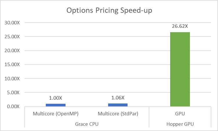
The key takeaway from this example is to expose parallelism in your application by default. The code should be written to express the available parallelism from the start. The ISO C++ code running on the same CPU and using the same compiler runs slightly better than the original because the compiler was able to better optimize the pure C++ code. That same code is over 26x faster when built for the NVIDIA Hopper GPU, thanks to the massive amount of available parallelism. All this was accomplished while reusing a significant amount of existing code.
With such significant speedups, time-consuming portfolio management workflows (like backtesting and simulations) become more practical. Traditionally, these have relied on modeling simplifications such as dimensionality reduction, Gaussian distributional assumptions, or other parsimonious representation choices to make the compute burden more manageable. Now, they can be done under more realistic conditions.
Parallel-first coding for optimal performance in quantitative finance
In conclusion, this post explores the transformative power of adopting a parallel-first approach in coding for quantitative finance using ISO C++. By refactoring existing code to leverage modern C++ features, such as spans and parallel algorithms, developers can seamlessly unlock the potential for parallelism on both multicore CPUs and GPUs.
Focusing on the rapid valuation of large options portfolios, the examples illustrate the substantial performance gains achievable through C++ standard parallelism. The comparison between the original OpenMP code and the ISO C++ parallel code running on both CPU and GPU platforms reveals significant speedups. This opens new possibilities for time-consuming portfolio management workflows such as backtesting and simulations.
The key takeaway is clear: writing code with inherent parallelism from the outset leads to more efficient and adaptable solutions. Embracing modern coding practices results in improved optimization by the compiler and, notably, a remarkable 26x acceleration when built for the NVIDIA Hopper GPU.
As developers venture into the realm of parallel programming, we encourage exploration and hands-on experience. The code samples available through NVIDIA/accelerated-quant-finance on GitHub, coupled with the NVIDIA HPC SDK, offer a practical avenue to delve into standard parallelism. While not intended for production use, these resources serve as valuable learning tools, empowering developers to integrate parallel-first principles into their own projects.
The future of coding in quantitative finance lies in embracing parallelism as a foundational principle. By doing so, developers pave the way for enhanced performance, greater adaptability, and the ability to navigate the evolving landscape of technology in the financial domain. Remember, in the realm of coding, the best code is always parallel-first.
