
Many GPU performance analysis tools are based on a capture and replay mechanism, where a frame is first captured (either in-memory or to disk), and then replayed multiple times to be profiled. Nsight Graphics: GPU Trace differs in that it directly profiles the frames emitted by a live application, with no constraint on subsequent frames to be identical. This approach makes the tool simpler than replay-based profilers, and therefore less likely to fail as graphics APIs evolve.
In a GDC 2019 talk, we showed how to apply the top-down P3 performance-triage method for optimizing any DX12 GPU workload using GPU Trace. One year later, with the release of Nsight Graphics 2020.2, the tool has evolved substantially. First, it now officially supports the Vulkan API (and all extensions, including VK_NV_ray_tracing). Second, it has a new “Advanced Mode”, which captures additional metrics over subsequent frames and presents them in a single view.
Specifically, in release 2020.2, the Advanced Mode metrics are:
- All of the SM Warp-Issue-Stall Reasons (“Why are my warp latencies high?”)
- All of the SM Warp-Launch-Stall Reasons (“Why is my warp occupancy low?”)
- The L1TEX Hit Rate (“Should I increase the spatial locality of my L1TEX accesses?”)
- A L2 Traffic Breakdown by Source Unit (“What are the GPU units that are causing most of the L2/VRAM memory traffic?”)
In this post, we show how to apply the P3 method using a performance-optimization example from Wolfenstein: Youngblood (VKR).
Capturing GPU Trace data with Advanced Mode Metrics
To capture GPU Trace data from a VK or DX12 app, you must first launch the app through Nsight Graphics and make sure that the tool is ready to capture. Multiple captures can then be taken from the same game session.
Launching an app through GPU Trace
To take a GPU Trace capture with the new advanced mode metrics:
- Launch Nsight Graphics 2020.2.
- Create a project (or use Quick Launch).
- Choose Connect.
- Under GPU Trace Launch options, for Metric Set, choose Advanced Mode Metrics.
- Set the path to your DX12 or VK EXE file.
- (Optional) Set the working directory and command line arguments.
- Choose Launch GPU Trace.
Here are some notes on using Advanced Mode Metrics:
- Advanced Mode Metrics assumes that the application is annotating its GPU workloads using performance markers (for example, PIXBeginEvent and PIXEndEvent for DX12). For recommendations on using perf markers, see the Optimizing Game Development with GPU Performance Events post.
- In this version of GPU Trace (2020.2), we recommend setting the frame count to 1 when Advanced Mode Metrics is enabled.
- As always, for GPU profiling, we recommend leaving Lock Clocks to Base enabled, which does the same as calling ID3D12Device::SetStablePowerState(TRUE). For more information, see SetStablePowerState.exe: Disabling GPU Boost on Windows 10 for more deterministic timestamp queries on NVIDIA GPUs.
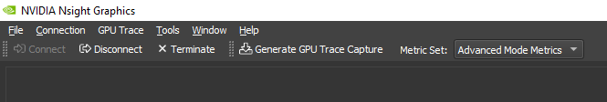
To make sure that GPU Trace has successfully attached itself to the application, you can ALT-Tab back to Nsight Graphics and check that you see the Generate GPU Trace Capture button:
Taking GPU Trace captures
When you are ready to take your first GPU Trace capture, perform the following steps:
- Make sure that your app is running in fullscreen mode and not hidden by any other window.
- Try to freeze the rendering (by pausing the game time, not moving the camera, and possibly disabling optimizations that amortize work over multiple frames).
- Press F11 to trigger a capture.
- Wait for at least 30 seconds and then ALT-Tab back to Nsight Graphics.
- If 30 seconds is not enough, wait for all the data to be captured and merged.
- Choose Open.
You can now take as many additional captures as needed to study the impact that any change has on GPU performance.
Applying the P3 method within GPU Trace
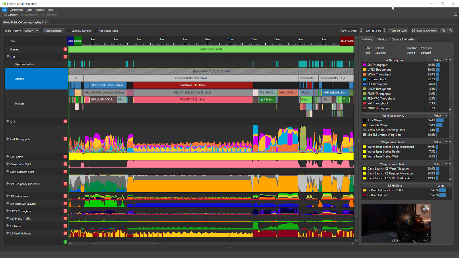
When GPU Trace opens the capture, the initial view looks like this, for a frame from Wolfenstein: Youngblood RTX:
Before taking our GPU Trace captures from a session of the game, we did the following by typing console variables in the game:
- Paused the game time
- Skipped all Ray-Tracing Acceleration Structure update/build commands
This is something you’d want to do anyway to compare two captures before and after making a change to the shaders. It’s even more important to remove frame-to-frame differences in the workloads when capturing advanced mode metrics, as these are captured from separate frames as the metric graphs.
Selecting a GPU workload to study
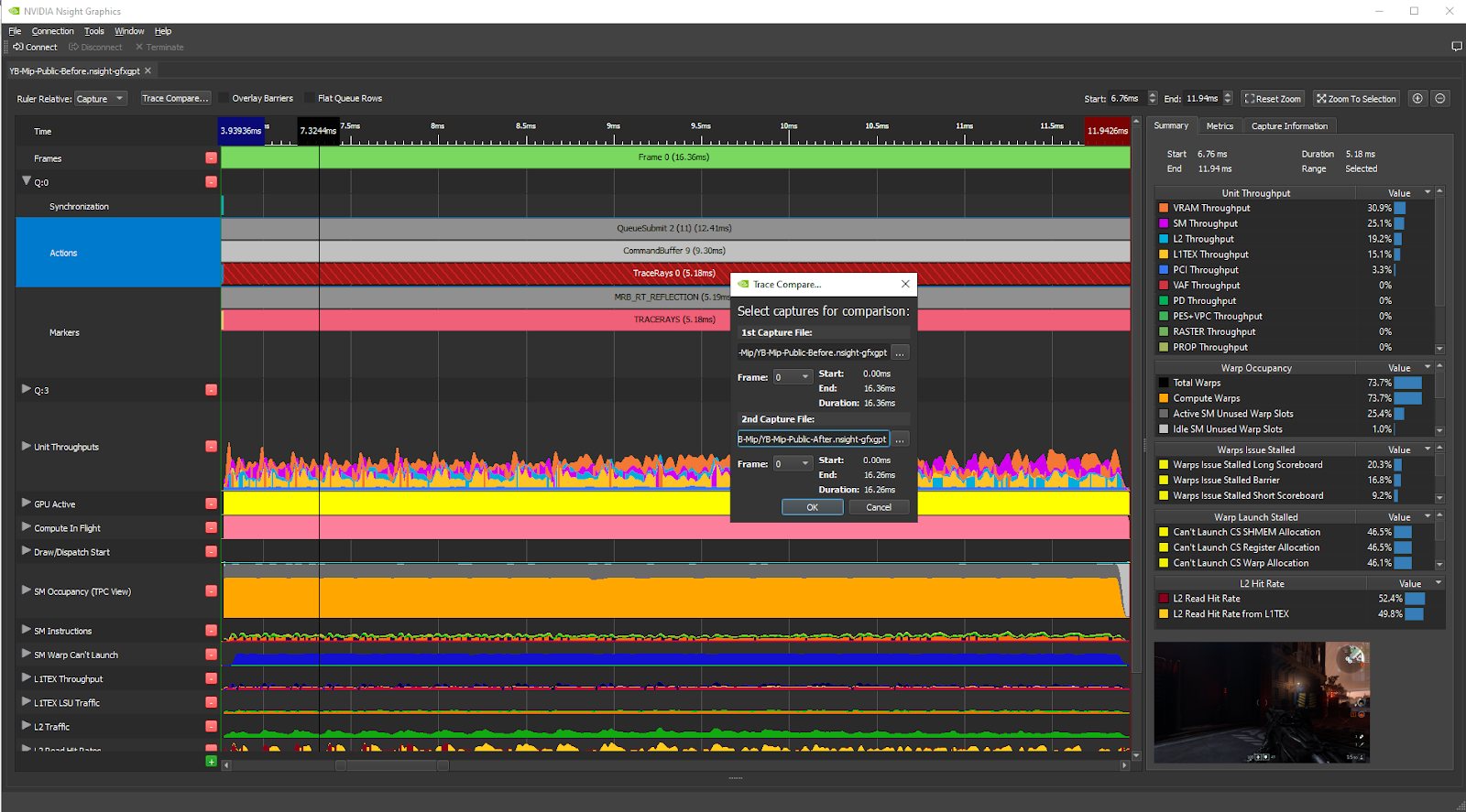
In this vkQueueSubmit call, the longest GPU workload is the Ray-Traced Reflections (MRB_RT_REFLECTIONS / TRACERAYS), taking 5.18 ms (42% of the main QueueSubmit call) in this frame on RTX 2080 with locked clocks.
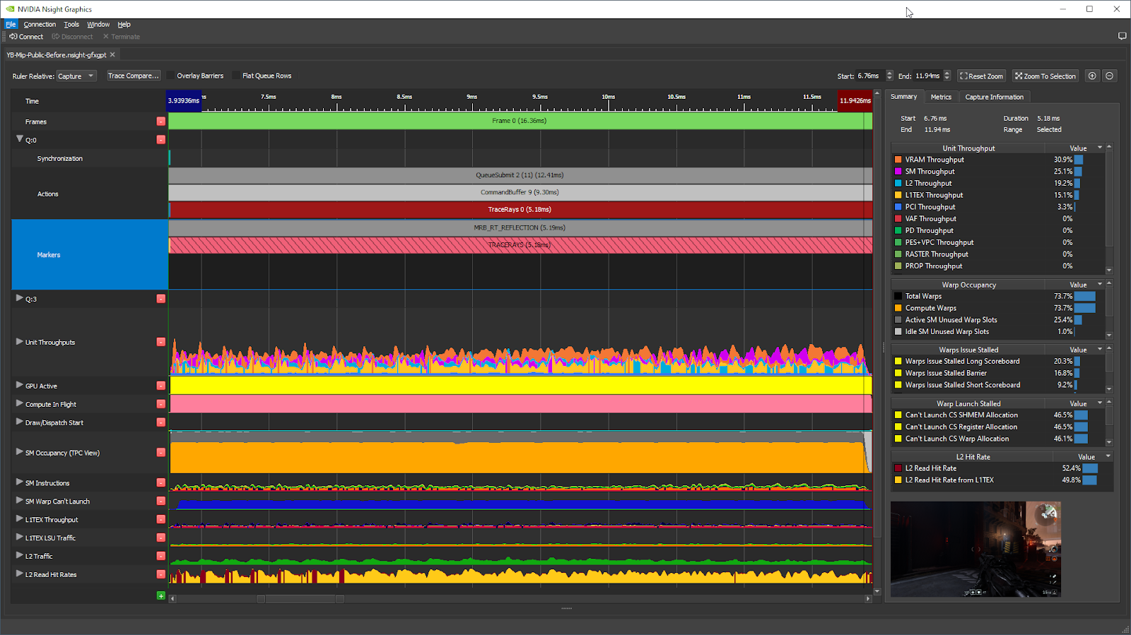
Double-click on this workload in the timeline, and the tool zooms in on that workload. The metrics in the right-side panel are updated to the associated time range:
Checking the GPU Active% metric
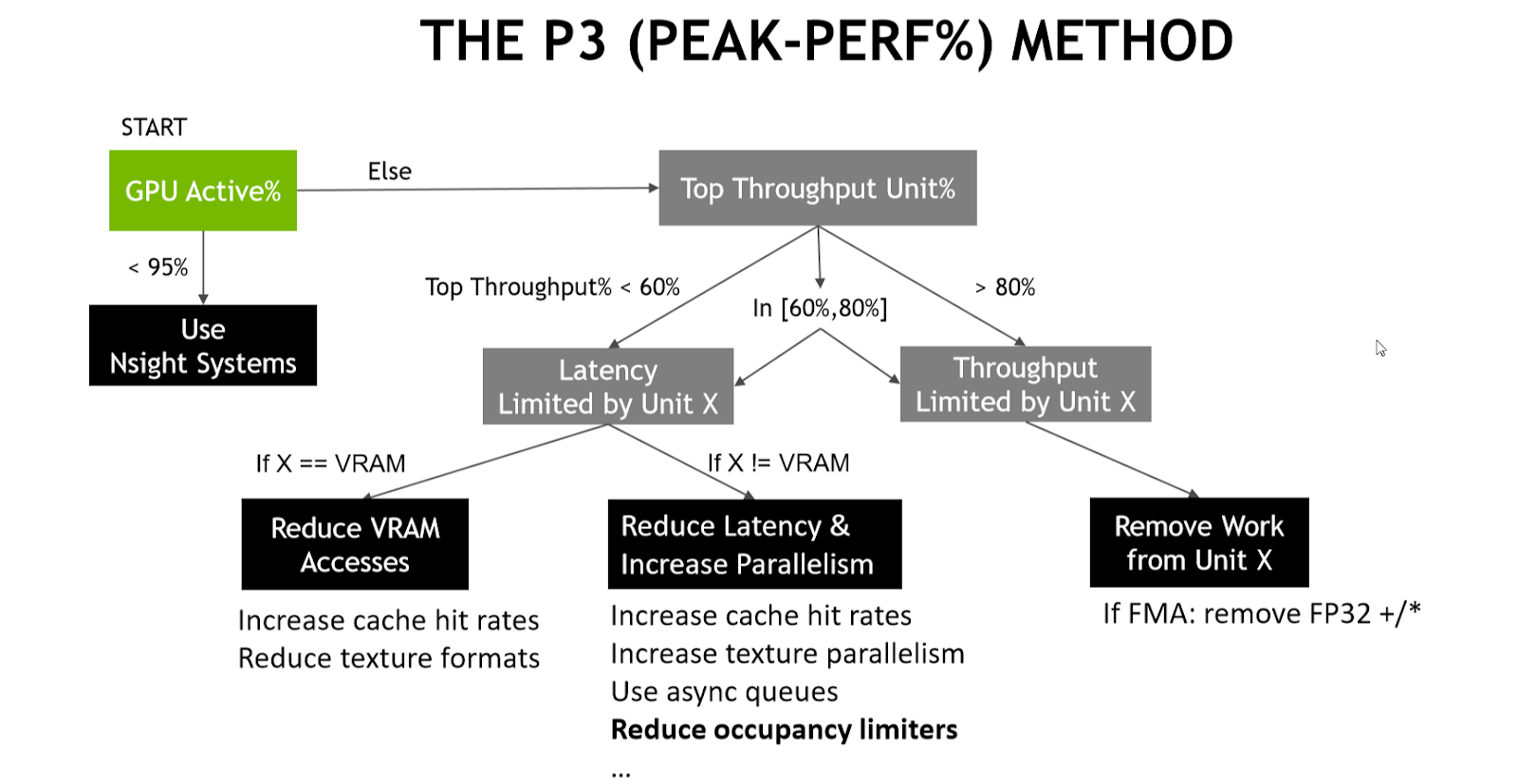
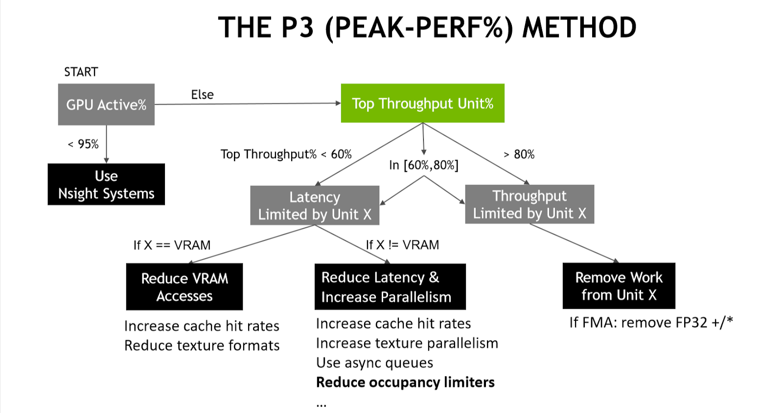
Now that we’ve selected a workload to focus on, we can apply the P3 (Peak Performance Percentage) method. The first step is to look at the GPU Active% metric:
This metric counts the percentage of the time that the Graphics/Compute Engine or the Copy Engines are active and GPU Trace displays it on the GPU Active metric graph. In this workload, GPU Active is 100.0% (as expected, as this is a single vkCmdTraceRaysNV):
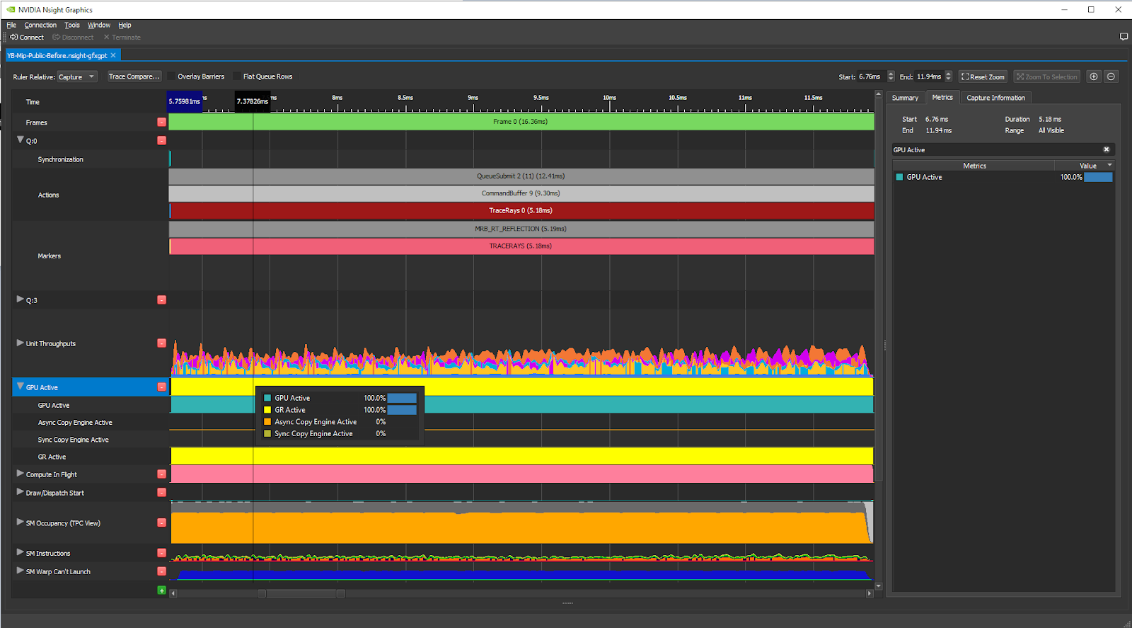
If that value was lower than 95%, we would know that there was 5% of the time where the GPU was fully idle. It may make sense to switch to using Nsight Systems to figure out what on the CPU side is limiting the performance.
Analyzing the top throughput units
The next step of the P3 method is to look at the Top Throughput metrics per GPU unit, sorted in decreasing order:
In GPU Trace, these are shown on the Unit Throughputs graph, and in the Summary section of the right pane:
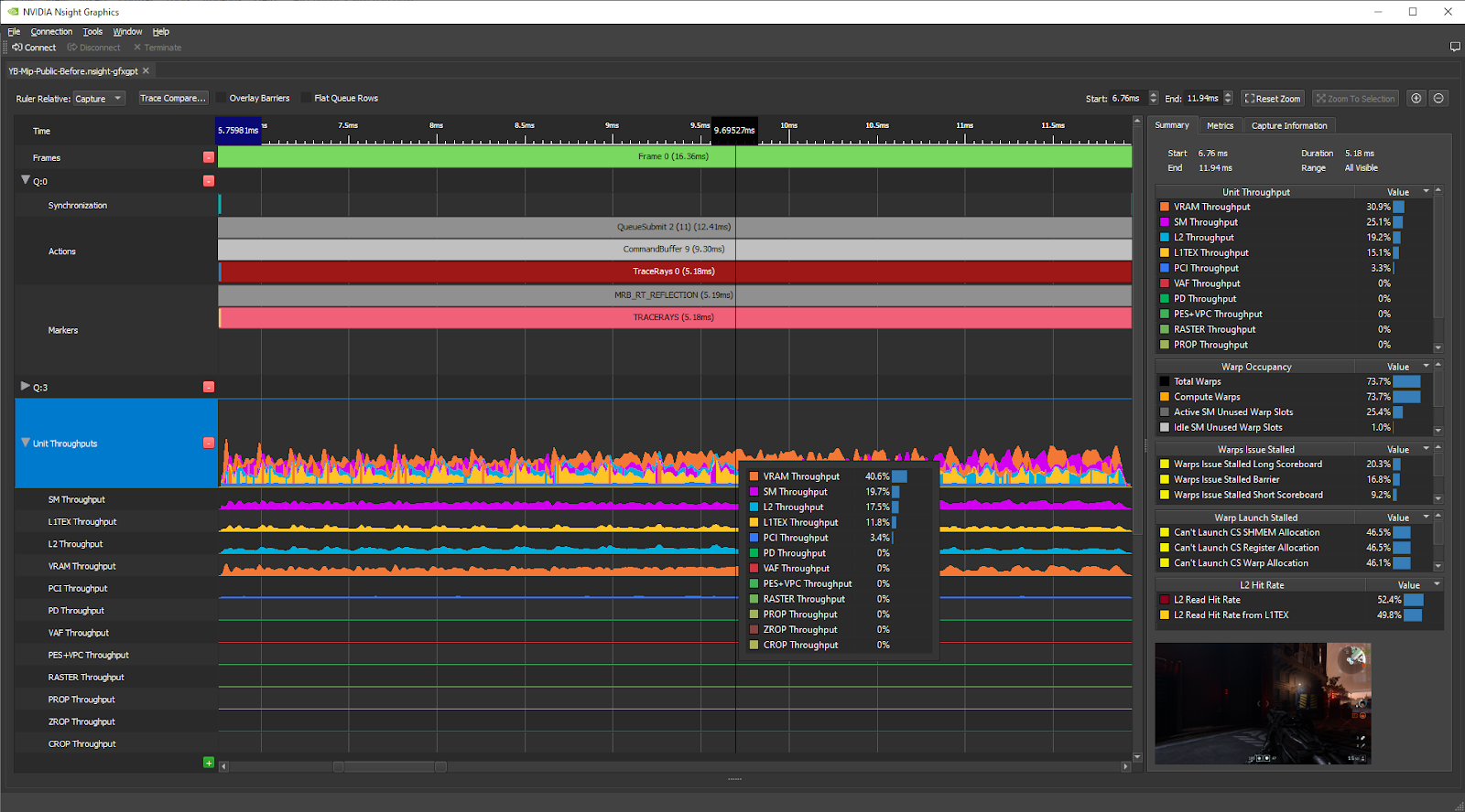
As we can see in the Summary tab, the Top Throughput (aka the Top SOL%) metrics per GPU unit for the RT Reflections workload are:
- VRAM: 30.9%
- SM: 25.1%
- L2: 19.2%
- L1TEX: 15.1%
- PCI: 3.3%
To copy and paste the metric names and values, select multiple rows, right-click, and choose Copy.
The top unit throughput% metric is the VRAM, and it’s very poor (<< 60%), so according to the P3 method, this workload is VRAM latency limited and you should reduce the number of VRAM accesses to speed it up.
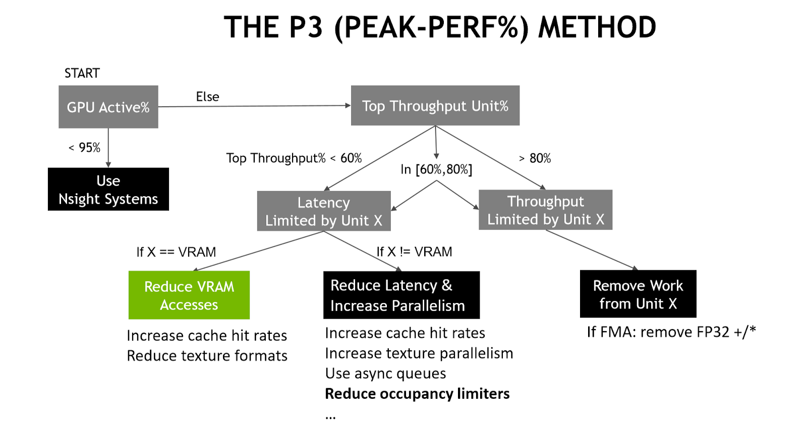
To achieve this, we want to know what kind of VRAM accesses are performed by this workload. On all NVIDIA GPUs after at least Fermi, all VRAM traffic goes through the L2 cache, so we can use L2 metrics to understand what requests are made to the VRAM.
Let’s use the new advanced mode metrics L2 Traffic Breakdown by Source Unit. Select the regime to study by clicking on it in the timeline. In the right pane, on the Metrics tab, type “srcunit” in the search box. The tool displays the metrics in decreasing order:
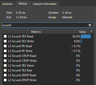
This L2 Srcunit TEX Read value means that 85.6% of the transferred bytes through the L2 cache originated from L1TEX reads. So we know that the best way to reduce the number of VRAM accesses is to reduce the number of read bytes requested by L1TEX.
Now, let’s take a look at the L1TEX and L2 hit rates by searching for “hit” on the Metrics tab:
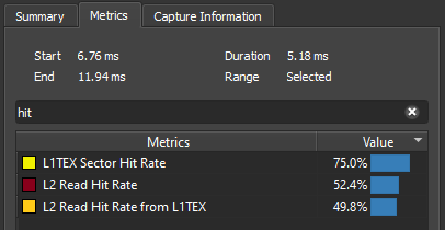
We see that the L1TEX Sector Hit Rate value is 75.0% and the L2 Read Hit Rate from L1TEX value is 49.8%. This poor L2 hit rate implies that the L1TEX reads are thrashing the L2 cache, which typically happens because the working set size of the simultaneously executing L1TEX reads is much greater than the L2 cache size.
Applying an optimization
It turned out that the hit shaders of this RT Reflections workload were fetching all 2D textures with the MIP level hardcoded to 0 for simplicity, because that was the easiest thing to do to get RT Reflections off the ground.
A well-known way to reduce the L2 working set size of the 2D texture fetches is to use mipmapping, because only the MIP levels that are accessed are resident in L2, and coarser levels occupy less bytes. Mipmaps were already populated by the engine, so all we needed to do was to replace the hard-coded MIP=0 with some dynamic MIP level.
As you can see in the presentation, Ray Traced Reflections in Wolfenstein: Youngblood (free GTC Digital account required), we ended up implementing a dynamic LOD approximation inspired by Texture Level of Detail Strategies for Real-Time Ray Tracing by Tomas Akenine-Möller, and the other authors. The MIP level approximation for this post is a function of:
- The distance from the ray origin to the camera origin
- The distance from the ray origin to the hit point
- The roughness of the material at the ray origin
- A constant texture LOD bias to further improve the performance
Before and after comparison
We implemented a dynamic MIP LOD in the hit shaders. After we were happy with it visually, we did a couple more GPU Trace captures from the same game session, still with paused game time, skipped RT acceleration structure updates, and static camera. The only change between the two captures was the MIP level calculation function (LOD=0 vs dynamic).
With the dynamic MIP LOD:
- The L2 Read Hit Rate from L1TEX improved greatly (from 50% to 83%), which makes sense because fetching coarser MIP levels reduces the size of the L1TEX working set resident in L2.
- The L1TEX Sector Hit Rate also slightly improved (from 75% to 80%), which makes sense because MIP mapping improves the locality of the accesses, where adjacent pixels fetch more adjacent texels.
- As a result, there was a 12% gain on the RT Reflections workload (5.18 -> 4.64 ms) in this frame.
Now, let’s compare the before and after captures directly within GPU Trace by choosing Trace Compare…:
Searching for “throughput” in the Metrics Search field in the right pane makes the tool show all per-unit and per-subunit throughput% metrics for the current workload:
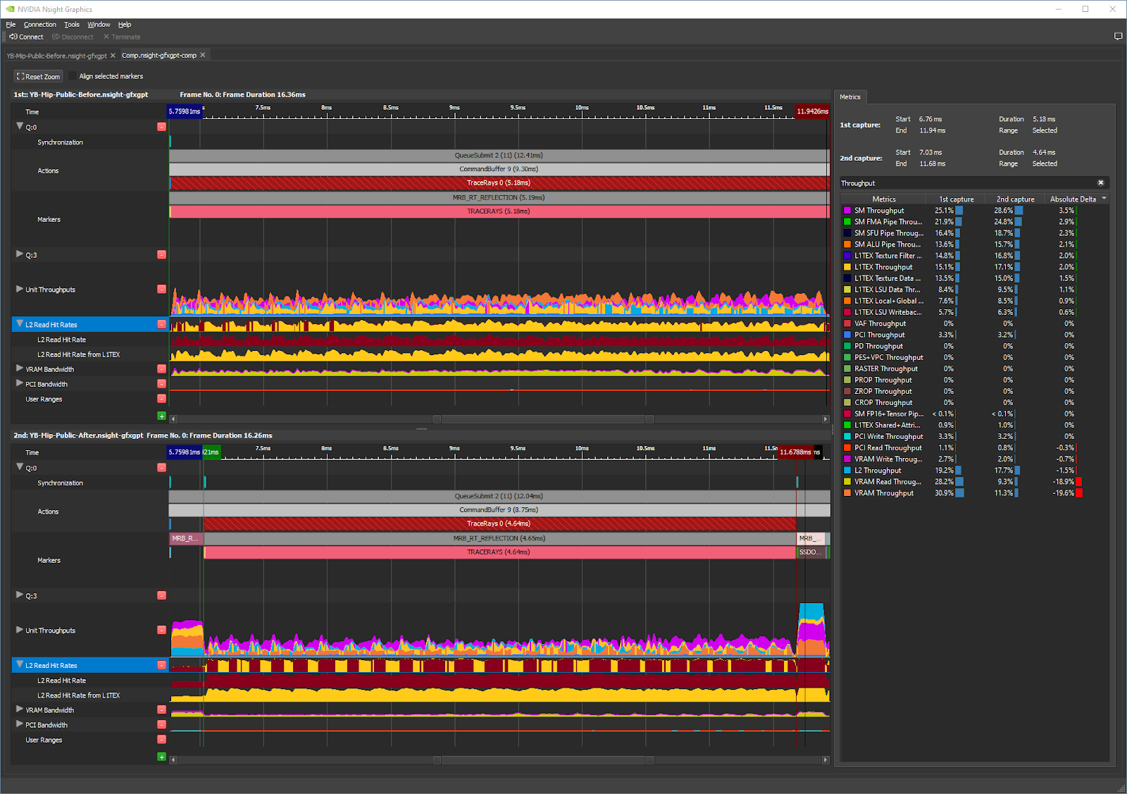
We see that the Top Unit Throughput metrics in the after capture are:
- SM: 28.6% (was 25.1%)
- L2: 17.7% (was 19.2%)
- L1TEX: 17.1% (was 15.1%)
- VRAM: 11.3% (was 30.9%)
- PCI: 3.2% (was 3.3%)
So the ray tracing workload was mainly VRAM latency–limited and no longer is, because the VRAM value is now far from being the top throughput metric. The L2 throughput has gone down slightly, which makes sense because there are less requests from L1TEX to L2, due to the slightly increased L1TEX hit rate.
The SM is now the top throughput unit, with a low SM throughput% (<<60%). To optimize it further, we should go down another branch of the decision tree of the P3 method and try to increase SM warp occupancy or decrease the SM warp latency. Increasing the SM warp occupancy earlier would have risked a slowdown due to increased VRAM pressure, while focusing on the high memory latency (and thus warp latency) had a greater chance to pay off.
Conclusion
If you are a graphics developer wanting to understand the performance limiters of a frame, you can start by launching your game with Nsight Graphics: GPU Trace with Advanced Mode Metrics enabled, and then using the P3 method to derive the main performance limiters of that workload.
- If you see drops in the GPU Active% graph, we recommend switching to Nsight Systems to figure out the reasons for the GPU being starved (which may be driver or OS overhead caused by certain graphics API calls, or just pure application-side CPU cycles). For more information, see Using Nsight Systems for Root-Cause Analysis of Game Stutters.
- If on the other hand, your GPU Active% graph looks good, you can go down the decision tree of the P3 method as we have shown in this post. For more examples of workloads with different limiters, see our GDC 2019 talk, Optimizing DX12/DXR GPU Workloads using Nsight Graphics: GPU Trace and the Peak-Performance-Percentage (P3) Method.
Acknowledgments
I’d like to thank Dana Elifaz and Assaf Pagi for having made it possible for the Advanced Mode Metrics to ship in GPU Trace, as well as Avinash Baliga, Aurelio Reis, and Sebastien Domine for their support.
