Introduction
Efficient pipeline design is crucial for data scientists. When composing complex end-to-end workflows, you may choose from a wide variety of building blocks, each of them specialized for a dedicated task. Unfortunately, repeatedly converting between data formats is an error-prone and performance-degrading endeavor. Let’s change that!
In this post series, we discuss different aspects of efficient framework interoperability:
- We start with this post discussing pros and cons of distinct memory layouts as well as memory pools for asynchronous memory allocation to enable zero-copy functionality.
- In the second post, we highlight bottlenecks occurring during data loading/transfers and how to mitigate them using Remote Direct Memory Access (RDMA) technology.
- In the third post, we dive into the implementation of an end-to-end pipeline demonstrating the discussed techniques for optimal data transfer across data science frameworks.
To learn more on framework interoperability, check out our presentation at NVIDIA’s GTC 2021 Conference.
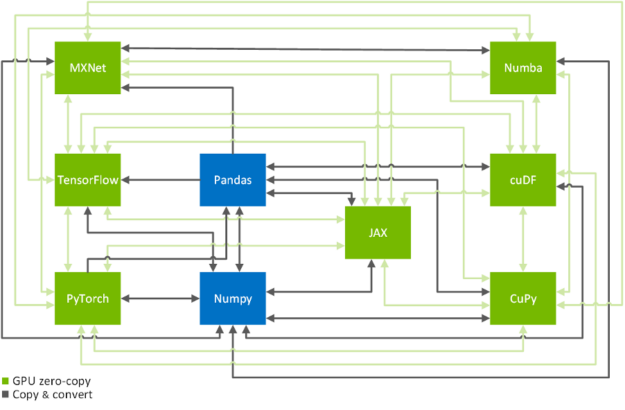
Zero-copy functionality is a crucial technique to efficiently copy data across GPU-accelerated data science frameworks: TensorFlow, PyTorch, MXNet, cuDF, CuPy, Numba, and JAX (see Figure 2). In the following, we will show you how to achieve that in a systematic manner. If you are only here to look up the commands on how to transfer data from one framework to another, you might want to have a look at this conversion table.
Memory layouts, data formats and memory pools
Memory Layouts
Before we start talking about how to copy data efficiently, let’s discuss how to store tabular data. In practice, all data formats inherit from one of the two major memory layouts known to computer scientists (see Figure 3):
- Array of Structures (AoS): A sequence of one or more data points x, y, z, … of potentially distinct type is represented as a structure S. Several instances of those data points are allocated as an array s of the new data type S. The original list of points x, y, z, … of the k-th instance is then accessed through the members s[k].x, s[k].y, s[k].z, … of the struct instance s[k].
- Structure of Arrays (SoA): Several instances of data points x, y, z, … are stored in separated arrays s_x, s_y, s_z, … The original points x, y, z, … of the k-th instance are then accessed by s_x[k], s_y[k], s_z[k], … Finally, these arrays can be interpreted as a single instance of a (merely virtually existing) structure, hence the name SoA.
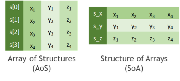
While the AoS layout looks more structured (pun intended) than SoA from a programmatic and abstraction point of view, it tends to be less suited for massively parallel algorithms in terms of achievable performance. This can be explained by a less efficient utilization of cache lines when consistently accessing a subset of the structure members, for example, during the reduction of values along one coordinate axis. You can even find cases in the literature where on-the-fly AoS-to-SoA conversion can significantly improve performance compared to plain processing in an AOS memory layout.
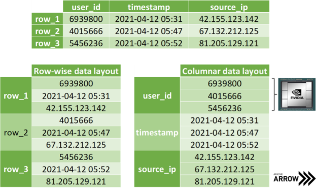
The SoA memory layout exhibits further advantages when copying coordinate-slices of the data. Assume you want to transfer all the x-coordinates at once, then you can access the corresponding array without the time-consuming slicing of members in the AoS layout. Even better, one can avoid allocating auxiliary memory when transferring data by simply exposing the address of the array in memory without copying a single byte. Apache Arrow is built on top of this methodology: storing data of distinct data types in different arrays for the discussed reasons (see Figure 4). Note that mainstream data science frameworks treat the entries of an array in the SoA layout as if they were stored in columns instead of rows, as depicted in Figure 3. However, this is merely a convention as we all know that virtually all memory is linearly ordered.
Data formats and zero-copy mechanism
In recent years, different libraries have been developed to address different needs. At the same time, data science pipelines have become more and more complex, requiring the usage of multiple libraries to accomplish a wide variety of tasks. Unfortunately, when these libraries were designed, interoperability between frameworks was not conceived as a top priority. As a result, there was a lack of standardized data formats suitable for data science tasks. Some people were concerned about data standards at that moment, like Wes McKinney, creator of the pandas project. In 2011, he published this post about a future roadmap for rich scientific data structures in Python.
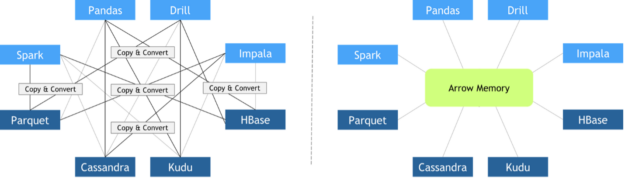
Since every library implemented its custom in-memory data layout and file formats, expensive copy-and-convert operations had to be performed when these libraries needed to collaborate. It was quite common that a significant portion of the total execution time was invested in meaningless copy-and-convert operations.
In October 2016, Apache Foundation released Arrow, a language-independent columnar-wise data format specification meant to deal efficiently with flat and hierarchical data on both CPUs and GPUs. Since then, many different frameworks have adopted it, facilitating zero-copy data exchange among them. Other key features of Apache Arrow columnar data format include:
- O(1) (constant-time) random access
- SIMD and vectorization-friendly
- Data adjacency for sequential access (scans)
- Relocatable without “pointer swizzling”, allowing for true zero-copy access in shared memory
Zero-copy mechanisms avoid unnecessary data transfers, reducing your application execution time drastically. Data science frameworks have added support to one or more of the following data formats: DLPack, CUDA Array Interface, and NumPy Array Interface.
DLPack is an open in-memory tensor structure for sharing tensors among frameworks. CUDA Array Interface and Numpy Array Interface are the de facto standards to exchange GPU and CPU array-like objects.
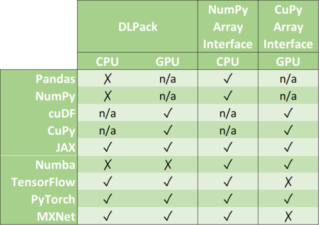
Please, note that some libraries like cuDF and CuPy exclusively run on GPU devices. Although it is possible to convert a NumPy array into a cuDF or CuPy object, we have marked its support as n/a because it requests data movement between host memory (CPU) and device memory (GPU).
In the following, we address memory layouts of the associated data objects in various frameworks, the efficient conversion of data objects using zero-copy, as well as the usage of a joint memory pool when mixing frameworks.
Memory pools
Memory allocations are expensive. They often impose global barriers, which block the remaining operations until the allocation is accomplished. Hence, repeatedly allocating memory in tight for-loops such as during the training of neural networks is prohibitive from a performance point of view. Modern data science and deep learning frameworks address this with dedicated memory pools. It is either preallocating a huge chunk of memory at the beginning of the program (for example, TensorFlow) or incrementally growing the pool using a few infrequent allocations (for example, PyTorch). Then, the preallocated memory is reused in a smart way by asynchronously assigning and retracting subsets of this memory range to/from whomever requests it. As an example, the RAPIDS Memory Manager (RMM) is a memory pool originally written for the RAPIDS data science framework. RMM facilitates blazingly fast host and device memory allocations. Mark Harris quantified the impact of RMM in this post: “We centralized memory management in cuDF by replacing all calls to cudaMalloc and cudaFree with RMM allocations. This was a lot of work, but it paid off. RMM calls are on the order of 1,000 times faster than cudaMalloc and cudaFree. The result was a 10x speedup for the mortgage demo.”
Several library-specific memory pools might compete for the same video RAM when combining distinct data science libraries. A straightforward workaround would be to limit the capacity of each memory pool to a fixed partition of the available memory. A better solution would be to use the same memory pool for all frameworks. Note that this does not necessarily mean that all frameworks must agree on the same memory pool implementation being shipped in their vanilla release. It is sufficient that all vendors agree to use an External Allocator Interface (EAI) for requesting and freeing memory in their frameworks.
void* allocate(std::size_t bytes, cudaStream_t stream)
void deallocate(void* p, std::size_t bytes, cudaStream_t stream)
Further advantages of an EAI are straightforward logging functionality, memory leak checking, as well as rate or resource limiting capabilities. For instance, the RAPIDS Memory Manager leverages unified memory to transparently oversubscribe GPU memory. The former translates into significantly reducing the chances of facing an Out of Memory error when working with huge datasets that do not fit in GPU memory.
The good news is that you can use RMM with CuPy and Numba by simply importing RAPIDS cuDF before importing everything else.
import cudf  # <= now RMM is the global memory pool
import cupy
import numba
Alternatively, you can combine Numba and RMM without using RAPIDS cuDF.
import rmm
from numba import cuda
cuda.set_memory_manager(rmm.RMMNumbaManager)
Conclusion
In this post of our framework interoperability series, you have learned about distinct memory layouts and how the Apache Arrow format can significantly speed up data transfers across distinct data science and machine learning frameworks such as TensorFlow, PyTorch, MXNet, cuDF, CuPy, Numba, and JAX. We have also discussed how asynchronous memory allocation facilitated by memory pools is crucial to avoid overheads as big as 90% of the overall runtime of your pipeline.
In the second part of the series, you will learn how Remote Direct Memory Access (RDMA) can be exploited to further accelerate data loading and data transfers in a multiple GPU setting.
