
Autonomous vehicles require fast and accurate perception of the surrounding environment in order to accomplish a wide set of tasks concurrently in real time. Systems need to handle the detection of obstacles, determine the boundaries of lanes, intersection detection, and sign recognition among many more functions over a large variety of environments, conditions, and situations and do this work quickly within the power limitations of an automotive setting. The DRIVE AGX platform has been purpose-designed to support these requirements.
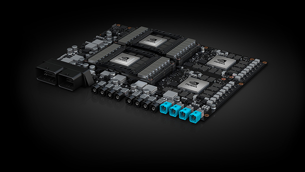
Powered by the Xavier SoC, the DRIVE platform features NVIDIA GPUs and a variety of other accelerators to spread the compute load, and is suitable for safety standards such as ISO 26262/ASIL-D, ISO/PAS 21448. These accelerators include the 64-bit ARM-based Octa-core CPU, an integrated Volta GPU, optional discrete Turing GPU, two deep learning accelerators (DLAs), multiple programmable vision accelerators (PVAs), and an array of other ISPs and video processors. This post dives into an application that runs two deep learning models concurrently to do both object recognition and ego-lane segmentation on an image. We released this application under the Apache License within the DL4AGX project, an open source project for tools and applications to ease development of deep learning enabled software for NVIDIA AGX platforms.
Easy Optimized Inference Pipelines Using TensorRT and DALI
TensorRT
TensorRT is NVIDIA’s high performance deep learning inference platform. It includes a deep learning inference optimizer and runtime that delivers low latency and high-throughput for deep learning inference applications. It allows the larger and more complex models to be practical in latency critical / compute limited applications such as autonomous driving.
We previously covered the process for optimizing a semantic segmentation model designed for object segmentation in autonomous driving scenarios by quantizing the network into an 8-bit integer representation (INT8) using TensorRT. It reduces the resources necessary to run inference, as well as leveraging specialized hardware within the GPU. This class of optimization is commonly used to reduce the latency of inference while still maintaining the accuracy of the model. It substantially helps fit all the computations needed in the narrow resource envelope available.
TensorRT 5.1 features the ability to not only optimize models for the GPUs available on DRIVE AGX systems but also the integrated Deep Learning Accelerators (DLA) within the Xavier SoC onboard at both FP16 and quantized INT8 operating precision. This allows developers to fully employ all the compute capability built into Xavier.
DALI
However, the task of running deep learning models is not limited to just the model itself. Preprocessing and post-processing represent key components of the total inference pipeline. The DALI library provides a collection of highly optimized image manipulation primitives and a graph based execution engine. This makes it easy to string together multiple operations implemented with highly efficient GPU kernels.
Managing compute across multiple devices can be difficult. Considerations such as synchronization, resource management, and computational dependencies need handling. The graph-based execution engine makes it natural to lay out these computations, provide data, and allow the library to worry about the dependency graph. resource management and data movement.
Merging DALI and TensorRT
TensorRT provides the fast inference needed for an autonomous driving application. DALI supplies the fast preprocessing as well as a simple way to manage the computational graph. It seems natural to use these toolkits together, accelerating the preprocessing and the inference.
We implement this integration via a DALI plugin which provides a TensorRT Operator. This operator places an optimized TensorRT engine directly into the DALI computational graph, consuming and producing the same data format as other DALI ops. Now DALI can manage the accelerated preprocessing, the optimized inference and the data transfer throughout the pipeline. We have released the source code for the TensorRT Inference Operator under the Apache License within the DL4AGX project. It has been verified on x86_64-linux, aarch64-linux (DRIVE AGX and Jetson AGX) and aarch64-qnx (DRIVE AGX). For more information, please checkout the README for the Plugin. Below we will look at an application using this operator.
Fast Concurrent Object Detection and Lane Segmentation on Heterogeneous Hardware Using DALI and TensorRT
Now we can have a fully accelerated inference pipeline. Let’s use this construction and TensorRT’s ability to run on both GPUs and DLAs along with DALI’s data management capabilities to run two models on the same data concurrently on separate accelerators, making more effective use of the Xavier SoC and its onboard accelerators. This allows us to overlap related tasks, such as simultaneous lane segmentation and object detection.
Concurrent inference on multiple different accelerators
For the simultaneous lane segmentation and object detection example, there is a common source image, but it needs to be preprocessed in seperate ways for each model. We therefore can potentially construct a computational graph as figure 1 shows:
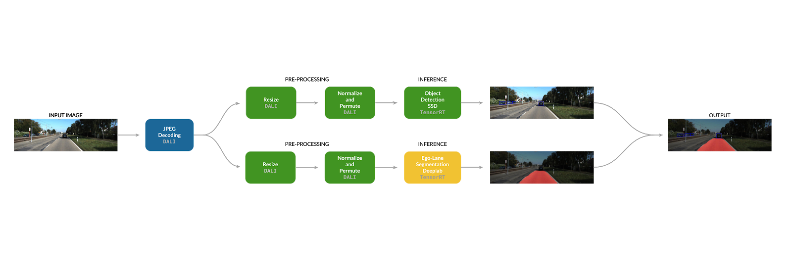
The preprocessing is done on the GPU using DALI’s kernels and inference for each arm runs on a different accelerator. This graph is what the inference application in the MultiDeviceInferencePipeline example implements.
Walking through the computational graph
This application uses a configuration file to set all the different settings of the computational graph. Going through this file is a good way to step through this graph node by node. The configuration file defines the input data and the output location for the annotated image. This acts as a stand-in for using an image stream as input, feeding the results into some high-level world representation or other A/V use case.
# From example_conf.toml
# Paths for I/O
input_image = "/path/to/input_image.jpg"
output_image = "/path/to/output_image.jpg"
Next one of the arms of the pipeline needs to be configured—in this case the segmentation arm. The model we chose for segmentation is designed to run entirely on the DLA (a list of supported layers by DLA can be referenced here to help determine model compatibility). You can see this arm of the graph is set to use DLA Core 1. You should also notice that the device (GPU) is also set to the device number of the iGPU, in our case, 1. This is the GPU Device used to interface with the DLA. On the Xavier SoC, the iGPU is the sole interface to the DLA and so must be targeted by TensorRT. However, the DLA still handles the computation. In addition, note the settings for configuring the DALI execution engine. In particular, take a look at the async execution setting, which means the two arms of the computational graph do not block each other.
# Configurations for the Segmentation Pipeline
[[inference_pipeline]]
name = "Segmentation"
device = 1           	# ID of GPU acting as DLA Bridge
dla_core = 1         	# Target device (DLA Core 1)
batch_size = 1
async_execution = true   # enable asynchronous execution of branches of pipeline
num_threads = 1      	# CPU Thread pool size
Below are the preprocessing settings for the segmentation arm of the graph. These values configure optimized GPU kernels that will resize and normalize the image for the input resolution of the TensorRT engine
[inference_pipeline.preprocessing]
# Image Pre-processing parameters
resize = [3, 240, 795]
mean = [0.0, 0.0, 0.0]
std_dev = [1.0, 1.0, 1.0]
Next is the TensorRT engine itself, which is consumed in the form of a serialized TensorRT engine (here it is saved to a file on the file system). The following sections detail information on the input and output heads of the network.
[inference_pipeline.engine]
# Path to TensorRT Engine
path = "experiments/deeplabv2_res18_small_240x795_int8_DLA.engine"

[[inference_pipeline.engine.inputs]]
# Name and shape of the model input tensor
name = "ImageTensor"
shape = [3, 240, 795]

[[inference_pipeline.engine.outputs]]
# Name and shape of the model output tensor
name = "logits/semantic/BiasAdd"
shape = [2, 15, 50]
That’s all the configuration needed for the segmentation arm. Next we add another [[inference_pipeline]] instance to configure the object detection. (Note: for the sake of clarity in the source code, the application is not fully generic; it does not handle an arbitrary set of pipelines. However, this is something that is pretty straightforward to implement within the existing code.)
Again we see the same high-level settings. Here we set dla_core set to -1, which means do not use the DLA for this engine and instead use the GPU (GPU Device 1, the iGPU on Xavier). Since the other network is running on the DLA, these two networks will actually be running on different devices even though they share a device number here.
[[inference_pipeline]]
name = "Object Detection"
device = 1             	# Target device (Xavier iGPU)
dla_core = -1          	# Disable DLA for this engine
batch_size = 1
async_execution = true 	# enable asynchronous execution of branches of pipeline
num_threads = 1        	# CPU Thread pool size
Once again we set the parameters for preprocessing, the path to the engine file, and its input and output heads.
[inference_pipeline.preprocessing]
# Image Pre-processing parameters
resize = [3, 300, 300]
mean = [127.5, 127.5, 127.5]
std_dev = [127.5, 127.5, 127.5]

[inference_pipeline.engine],
# Path to TensorRT Engine
path = "experiments/SSD_resnet18_kitti_int8_iGPU.engine"

[[inference_pipeline.engine.inputs]]
# Name and shape of the model input tensor
name = "Input"
shape = [3, 300, 300]
Here we see that this network has more than one output head. This is a result of the TensorRT NMS plugin but DALI is able to handle this accordingly.
[[inference_pipeline.engine.outputs]]
# Name and shape of the model output tensor
name = "NMS"
shape = [1, 100, 7]

[[inference_pipeline.engine.outputs]]
# Name and shape of additional model output tensor (specific to TRT NMS Plugin)
name = "NMS_1"
shape = [1, 1, 1]
We also see here the use of a custom plugin which implements a FlattenConcat Operator, used by the SSD Network.
[[inference_pipeline.engine.plugins]]
# Path to TensorRT Plugin for FlattenConcat Op (see //plugins/TensorRT/FlattenConcat)
path = "/bazel-bin/plugins/FlattenConcatPlugin/libflattenconcatplugin.so"
Taken together the whole configuration file represents the full pipeline shown in the diagram above.
Generic Inference Pipeline Implementation
Throughout this blog post, we have been continually returning to this basic preprocessing -> inference subgraph primitive. Now let’s look at how a generic version of this primitive can be implemented using DALI and TensorRT together. This DALITRTPipeline class gets configured and instantiated for each inference pipeline entry in the configuration file and serves as an encapsulation of the subgraph, taking raw decoded jpegs in and returning the results from the model. This constructor contains the main logic around creating this basic subgraph (the remaining components being mostly small wrappers around DALI).
// From DALITRTPipeline.cpp
DALITRTPipeline::DALITRTPipeline(const std::string pipelinePrefix,
                                preprocessing::PreprocessingSettings preprocessingSettings,
                                std::string TRTEngineFilePath,
                                std::vector pluginPaths,
                                std::vector engineInputBindings,
                                std::vector engineOutputBindings,
                                const int deviceId,
                                const int DLACore,
                                const int numThreads,
                                const int batchSize,
                                const bool pipelineExecution,
                                const int prefetchQueueDepth,
                                const bool asyncExecution)
{
The construction of the pipeline begins here, with a new DALI pipeline, to which we add an input node and the preprocessing steps of the arm.
this->inferencePipeline = new dali::Pipeline(batchSize, numThreads,
                                               deviceId, seed,
                                               pipelineExecution,
                                               prefetchQueueDepth,
                                               asyncExecution); //max_num_stream may become useful here
   //Hardcoded Input node
   const std::string externalInput = "decoded_jpegs";
   this->inputs.push_back({externalInput, "cpu"});
   this->inferencePipeline->AddExternalInput(externalInput);
   const std::vector<std::pair<std::string, std::string>> preprocessingOutputNodes = {std::make_pair("preprocessed_images", "gpu")};
   //Single function to append the preprocessing steps to the pipeline (modify this function in preprocessingPipeline/pipeline.h to change these steps)
   preprocessing::AddOpsToPipeline(this->inferencePipeline, pipelinePrefix,
                                   this->inputs[0], preprocessingOutputNodes,
                                   preprocessingSettings, true);
You can see the actual operations below. First, the image is resized to an input size of the model, then normalized. Both of these operations are handled by the GPU by default via DALI.
//From preprocessing.h
inline void AddOpsToPipeline(dali::Pipeline* pipe,
                           const std::string prefix,
                           const std::pair<std::string, std::string> externalInput,
                           const std::vector<std::pair<std::string, std::string>> pipelineOutputs,
                           const preprocessing::PreprocessingSettings& settings,
                           bool gpuMode)
{
   int nChannel = settings.imgDims[0]; //Channels
   int nHeight = settings.imgDims[1];  //Height
   int nWidth = settings.imgDims[2];   //Width
   std::string executionPlatform = gpuMode ? "gpu" : "cpu";
   pipe->AddOperator(
       dali::OpSpec("Resize")
          .AddArg("device", executionPlatform)
          .AddArg("interp_type", dali::DALI_INTERP_CUBIC)
          .AddArg("resize_x", (float) nWidth)
          .AddArg("resize_y", (float) nHeight)
          .AddArg("image_type", dali::DALI_RGB)
          .AddInput("decoded_jpegs", executionPlatform)
          .AddOutput("resized_images", executionPlatform),
       prefix + "_Resize");
   pipe->AddOperator(
       dali::OpSpec("NormalizePermute")
          .AddArg("device", executionPlatform)
          .AddArg("output_type", dali::DALI_FLOAT)
          .AddArg("mean", settings.imgMean)
          .AddArg("std", settings.imgStd)
          .AddArg("height", nHeight)
          .AddArg("width", nWidth)
          .AddArg("channels", nChannel)
          .AddInput("resized_images", executionPlatform)
          .AddOutput(pipelineOutputs[0].first, pipelineOutputs[0].second),
       prefix + "_NormalizePermute");
}
Finally, we add TensorRT engine to the pipeline using the TensorRT Plugin for DALI. The engine is ingested from a serialized TensorRT engine. We set inputs, outputs and plugins, and settings for the engine and inference runtime at this point.
//Read in TensorRT Engine
std::string serializedEngine;
utils::readSerializedFileToString(TRTEngineFilePath, serializedEngine);
dali::OpSpec inferOp("TensorRTInfer");
inferOp.AddArg("device", "gpu")
.AddArg("inference_batch_size", batchSize)
.AddArg("engine", serializedEngine)
.AddArg("plugins", pluginPaths)
.AddArg("num_outputs", engineOutputBindings.size())
.AddArg("input_nodes", engineInputBindings)
.AddArg("output_nodes", engineOutputBindings)
.AddArg("log_severity", 3);
The choice of using the DLA or the GPU is actually an argument of the TensorRT operator provided by our plugin.
// Decide whether to use a DLA for the engine or not
if (DLACore >= 0)
{
inferOp.AddArg("use_dla_core", DLACore);
}
for (auto& in : preprocessingOutputNodes)
{
inferOp.AddInput(in.first, "gpu");
}
for (auto& out : engineOutputBindings)
{
inferOp.AddOutput(out, "gpu");
this->outputs.push_back({out, "gpu"});
}
std::cout << "Registering " << pipelinePrefix << " TensorRT Op" << std::endl;
this->inferencePipeline->AddOperator(inferOp);
}
}
Tying the Pipeline Together
Given this simple primitive and its configuration, we now construct the full multi-device pipeline.
The first stage is to load in an image from the file system—in a real autonomous vehicles application, this will likely be an image stream. The image starts by being decoded and two copies made via DALI to feed each arm of the pipeline.
std::cout << "Load JPEG images" << std::endl; dali::TensorList JPEGBatch; utils::makeJPEGBatch(settings.inFiles, &JPEGBatch, settings.batchSize); JPEGPipeline.SetPipelineInput(JPEGBatch); JPEGPipeline.RunPipeline(); std::vector<dali::TensorList*> detInputBatch; std::vector<dali::TensorList*> segInputBatch; JPEGPipeline.GetPipelineOutput(detInputBatch, segInputBatch);
We set the images inputs into the main arms of the pipeline from the point where the image has been decoded. DALI handles all the memory management and transfer of data between CPU and GPU.
   // Load this image into the pipeline (note there is no cuda memcpy yet as
   // JPEG decoding is done CPU side, DALI will handle the memcpy between ops
   std::cout << "Load into inference pipelines" << std::endl;
   detPipeline.SetPipelineInput(detInputBatch);
   segPipeline.SetPipelineInput(segInputBatch);
The actual execution starts after setting the inputs. The arms run asynchronously, so operations in one arm will not block operations in the other arm. The GetPipelineOutput calls serve as a barrier, synchronizing the two arms before post processing.
// Run the inference pipeline on both the GPU and DLA // While this is done serially in the app context, when the pipelines are built // with AsyncExecution enabled (default), the pipelines themselves will run concurrently std::cout << "Starting inference pipelines" << std::endl; detPipeline.RunPipeline(); segPipeline.RunPipeline(); // Now setting a blocking call for the pipelines to synchronize the pipeline executions std::cout << "Transferring inference results back to host for postprocessing" << std::endl; std::vector<dali::TensorList*> detPipelineResults; std::vector<dali::TensorList*> segPipelineResults; detPipeline.GetPipelineOutput(detPipelineResults); segPipeline.GetPipelineOutput(segPipelineResults);
Finally, data is copied back and is unwrapped for post-processing and ultimately visualization (in a full AV application it may go on to update the world representation).
// Copy data back to host
std::vector detNMSOutput(conf::bindingSize(settings
.pipelineBindings[kDET_PIPELINE_NAME]
.outputBindings["NMS"]),
0);
std::vector detNMS1Output(conf::bindingSize(settings
.pipelineBindings[kDET_PIPELINE_NAME]
.outputBindings["NMS_1"]),
0);
std::vector segOutput(conf::bindingSize(settings
.pipelineBindings[kSEG_PIPELINE_NAME]
.outputBindings["logits/semantic/BiasAdd"]),
0);
utils::GPUTensorListToRawData(detPipelineResults[0], &detNMSOutput);
utils::GPUTensorListToRawData(detPipelineResults[1], &detNMS1Output);
utils::GPUTensorListToRawData(segPipelineResults[0], &segOutput);
Results
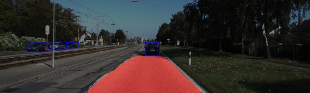
Figure 2 shows an example of what the system produces, an annotated image with detections and a lane segmentation. Instead of outputting an image, this pipeline can instead feed other components of the self driving system in a more real world application.
Using DALI and TensorRT to accelerate inference generates significant performance speedups in both the actual model execution and the preprocessing by fully utilizing the hardware onboard the DRIVE AGX, as shown in figure 3.

This post has investigated using DALI and TensorRT as a way to more simply manage a heterogeneous compute pipeline. However, we also see significant performance improvements by using these two libraries together. We benchmarked a ResNet-18 model pipeline implemented with DALI and TensorRT on the Xavier SoC. Inference via TensorRT is performed over GPU in this case. We show a 1.57x speedup due to the use of GPU accelerated preprocessing and a 3.5x increase in performance by using quantized INT8 over FP32 execution of the model.
In addition to better utilizing the variety of accelerators on board the Xavier SoC by using DALI and TensorRT together,we also improve the performance of the computation itself.
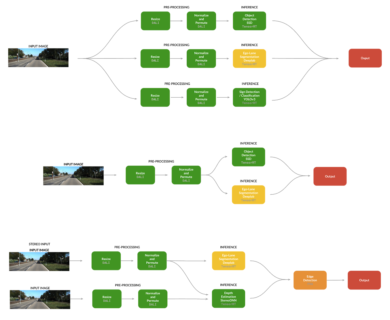
Extending This Concept
The basic two model example, as seen earlier in figure 1, shows the potential of this approach to inference. From here one could extend wider, including more models in the graph, or use different input setups like stereo image pairs, as shown in figure 4. There is potential to further extend DALI to have operators leveraging other accelerators on Xavier like the PVA. With the generic components we detailed above, implementing these varied systems in a fashion that fully leverages the compute capabilities of the DRIVE AGX does not take much effort.
Trying it for yourself
The application source code, recipes for training the models and source code for the TensorRT DALI Integration are open source and released in the DL4AGX repo within the MultiDeviceInferencePipeline directory and has been tested on DRIVE AGX (Both QNX and Linux), Jetson AGX and x86_64 (with multiple GPUs instead of GPU + DLA). You’ll find detailed instructions on how to train the Object Detection and Lane Segmentation models on the KITTI dataset, cross compile all of the applications for the target hardware and convert those models to TensorRT Engines for use in this pipeline as well as the actual usage of the application.
Creating and Running Applications on DRIVE AGX
The DL4AGX project continues to develop deep learning tools and applications for the various AGX platforms. It is based around a containerized build infrastructure using Bazel and Docker that allows the cross compilation of these applications and tools to be really simple and easy to set up. Supported environments include ones based on the DRIVE AGX PDKs and Jetpack/Jetson AGX. Keep an eye on this repo for new tools and applications that should help developing Deep Learning applications for AGX platforms a lot simpler.
References
[Geiger et al. 2013] Geiger, A., Lenz, P., Stiller, C., & Urtasun, R. (2013). Vision meets robotics: The KITTI dataset. The International Journal of Robotics Research, 32(11), 1231-1237.
[Chen et. al 2017] Chen, L. C., Papandreou, G., Kokkinos, I., Murphy, K., & Yuille, A. L. (2017). Deeplab: Semantic image segmentation with deep convolutional nets, atrous convolution, and fully connected crfs. IEEE transactions on pattern analysis and machine intelligence, 40(4), 834-848.
[Liu et. al 2016] Liu, W., Anguelov, D., Erhan, D., Szegedy, C., Reed, S., Fu, C. Y., & Berg, A. C. (2016, October). Ssd: Single shot multibox detector. In European conference on computer vision (pp. 21-37). Springer, Cham.
[Smolyanskiy et al. 2018] Smolyanskiy, N., Kamenev, A., & Birchfield, S. (2018). On the importance of stereo for accurate depth estimation: An efficient semi-supervised deep neural network approach. In Proceedings of the IEEE Conference on Computer Vision and Pattern Recognition Workshops (pp. 1007-1015).
[Redmon et. al. 2018] Redmon, J., & Farhadi, A. (2018). Yolov3: An incremental improvement. arXiv preprint arXiv:1804.02767.