During the 2020 NVIDIA GPU Technology Conference keynote address, NVIDIA founder and CEO Jensen Huang introduced the new NVIDIA A100 GPU based on the NVIDIA Ampere GPU architecture.
In this post, we detail the exciting new features of the A100 that make NVIDIA GPUs an ever-better powerhouse for computer vision workloads. We also showcase two recent CV research projects from NVIDIA Research, Hierarchical Multi-Scale Attention for Semantic Segmentation and Bi3D: Stereo Depth Estimation via Binary Classifications, and show how they benefit from the A100.
The NVIDIA A100 is the largest 7nm chip ever made with 54B transistors, 40 GB of HBM2 GPU memory with 1.5 TB/s of GPU memory bandwidth. The A100 offers up to 624 TF of FP16 arithmetic throughput for deep learning (DL) training, and up to 1,248 TOPS of INT8 arithmetic throughput for DL inference. At a high level, the NVIDIA A100 is packed with a suite of exciting new features:
- Multi-Instance GPU (MIG) allows the A100 Tensor Core GPU to be securely partitioned into as many as seven separate GPU instances for CUDA applications
- Third-generation Tensor Cores with TensorFloat 32 (TF32) instructions which accelerate processing of FP32 data
- Third-generation NVLink at 10X the interconnect speed of PCIe gen 4
- For CV workloads, the number of video decoders in the A100 went up dramatically to five compared to one video decoder on the V100. It also includes five new hardware JPEG decoder engines and new improved hardware for optical flow.
For a deeper dive into the NVIDIA Ampere architecture, see NVIDIA Ampere Architecture In-Depth and the A100 white paper.
CV research at NVIDIA
At CVPR 2020, NVIDIA researchers are presenting 15 research papers. In this post, we showcase two recent CV research projects at NVIDIA:
- Hierarchical Multi-Scale Attention for Semantic Segmentation
- NVIDIA A100 Tensor Core GPU Architecture
Hierarchical Multi-Scale Attention for Semantic Segmentation
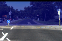
There’s an important technology that is commonly used in autonomous driving, medical imaging, and even Zoom virtual backgrounds: semantic segmentation. That’s the process of labelling pixels in an image as belonging to one of N classes (N being any number of classes), where the classes can be things like cars, roads, people, or trees. In the case of medical images, classes correspond to different organs or anatomical structures.
NVIDIA Research is working on semantic segmentation because it is a broadly applicable technology. We also believe that the techniques discovered to improve semantic segmentation may also help to improve many other dense prediction tasks, such as optical flow prediction (predicting the motion of objects), image super-resolution, and so on.
Multi-scale inference is commonly used to improve the results of semantic segmentation. Multiple images scales are passed through a network and then the results are combined with averaging or max pooling.
In the Hierarchical Multi-Scale Attention for Semantic Segmentation paper, we present an attention-based approach to combining multi-scale predictions. We show that predictions at certain scales are better at resolving some failure modes, and that the network learns to favor those scales for such cases in order to generate better predictions. Our attention mechanism is hierarchical, which enables it to be roughly 4x more memory efficient to train than other recent approaches. In addition to enabling faster training, this allows us to train with larger crop sizes which leads to greater model accuracy.
We demonstrate the result of our method on two datasets: Cityscapes and Mapillary Vistas. For Cityscapes, which has many weakly labelled images, we also leverage auto-labelling to improve generalization. Using this approach, we achieve new state-of-the-art results in both Mapillary (61.1 IOU val) and Cityscapes (85.1 IOU test).
Bi3D: Stereo Depth Estimation via Binary Classifications
Stereo-based–depth estimation is a cornerstone of computer vision, with state-of-the-art methods delivering accurate results. Several applications, such as autonomous navigation, do not always require centimeter-accurate depth, but have strict latency requirements.
In fact, the required accuracy, latency, and the range of interest for depth estimation varies with the task at hand. Highway driving, for instance, requires a longer range of measurements at extremely low latencies, but can deal with coarsely quantized depth. It’s more important to detect an obstacle that is roughly 80 meters within milliseconds, than finding out 10 milliseconds later that it’s exactly 81.2 meters away. Parallel parking, on the other hand, does not need extremely fast results, but the tolerance for error is much lower. Hence, there is a need for a flexible, stereo depth–estimation approach that allows such trade-offs at inference time.
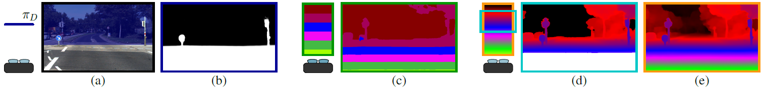
Bi3D offers a solution to this problem. Given a strict time budget, Bi3D can detect objects closer than a given distance in as little as a few milliseconds (Figure 1(b)). This binary depth yields 1-bit information at extremely low latencies. Combining binary decisions at several depths allows you to estimate depth with arbitrarily coarse quantization (Figure 1(c)), and complexity linear with the number of quantization levels. Bi3D can also use the budget of quantization levels to get continuous (high-quality depth) in a specific depth range (Figure 1(d)). For standard stereo (that is, continuous depth on the whole range, Figure 1(e)), Bi3D is close to or on par with state-of-the-art, finely tuned, stereo methods.
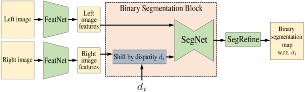
The core of the method is Bi3DNet, a network that takes as input the left image and the right image, and a candidate disparity \(d_{i}\) (Figure 2). The output is a binary segmentation probability map that segments the range into two: disparities that are larger or smaller than \(d_{i}\). Testing even a single disparity \(d_{i}\)tells you if the disparity at any pixel is smaller or larger than\(d_{i}\). By testing multiple such disparities, you can estimate the depth at which a pixel switches from being in-front to being behind, that is, the depth for that pixel. For more information, see the NVlabs/Bi3D GitHub repo.
A100 training results
In this section, we discuss the training performance of the semantic segmentation and Bi3D networks:
- TF32: speeding up FP32 effortlessly
- Automatic mixed precision training
TF32: Speeding up FP32 effortlessly
Ampere third-generation Tensor Cores support a novel math mode: TF32. TF32 is a hybrid format defined to handle the work of FP32 with greater efficiency. Specifically, TF32 uses the same 10-bit mantissa as FP16 to ensure accuracy while sporting the same range as FP32, thanks to using an 8-bit exponent. By striking a balance between accuracy and efficiency, TF32 running on Tensor Cores in A100 GPUs can provide up to 10x throughput compared to single-precision floating-point math (FP32) on Volta GPUs.
On Ampere Tensor Cores, TF32 is the default math mode for all DL workloads, as opposed to FP32 on Volta/Turing GPUs. Internally, when operating in TF32 mode, Ampere Tensor Cores accept two FP32 matrices as inputs but internally carry out matrix multiplication in TF32. The result is added to an FP32 accumulator.
To make use of TF32 on A100, write and run your code as you would normally do with FP32 data type. The rest is handled automatically by the DL frameworks. Starting from version 20.06, NVIDIA DL framework containers for TensorFlow, PyTorch, and MXNet support TF32 on A100 and can be downloaded freely from the NVIDIA NGC.
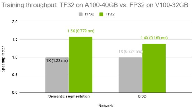
In Figure 3, we show the throughput when training the multi-scale attention semantic segmentation network and the Bi3D network with FP32 on V100 and TF32 on A100. Without any code change, TF32 offers a 1.6X and 1.4X speedup, respectively.
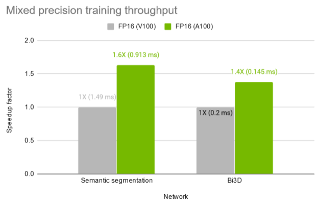
Automatic mixed precision training
TF32 is designed to bring the processing power of NVIDIA Tensor Core technologies to all DL workloads without any code change required from developers.
However, for more savvy researchers who wish to unlock the highest throughput, mixed precision training, which uses mostly FP16 but also FP32 data type where necessary, remains the most performant option.
Automatic mixed precision (AMP) training on NVIDIA GPUs can be enabled easily with either no code change (when using the NVIDIA NGC TensorFlow container) or with just a few lines of extra code. When operating in FP16 mode, Ampere Tensor Cores accept FP16 matrices instead, and accumulate in an FP32 matrix. FP16 mode on Ampere provides twice the throughput compared to TF32.
Figure 4 shows the throughput when training the multi-scale attention semantic segmentation network and the Bi3D network with mixed precision on V100 and A100. AMP on A100 offers a 1.6X and 1.4X speedup respectively compared to AMP on a V100 32 GB GPU.
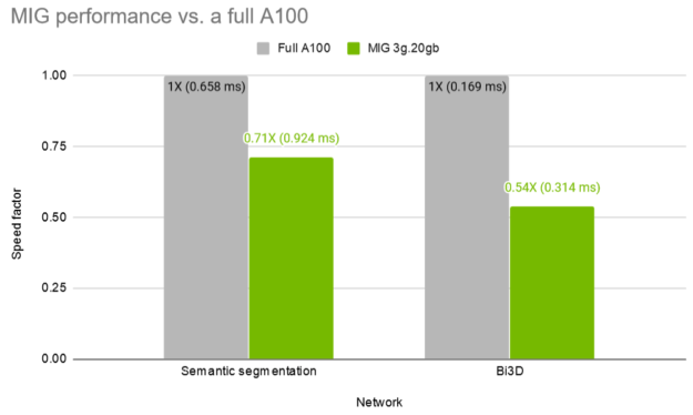
Multi-instance GPU for training
Multi-Instance GPU (MIG) partitions a single NVIDIA A100 GPU into as many as seven independent GPU instances. They run simultaneously, each with its own memory, cache, and streaming multiprocessors (SM). That enables the A100 GPU to deliver guaranteed quality-of-service (QoS) at up to 7x higher utilization compared to prior GPUs.
For heavy training workloads, such as multi-scale attention semantic segmentation and Bi3D network training, you can create two so-called MIG 3g.20gb instances, each with 20 gigabytes (GB) of GPU memory and 42 SMs. This allows two researchers to run independent investigations without having to worry about interfering with one another in terms of memory and computation.
In this section, we experiment with two parallel training workloads on an A100 GPU that has been configured into 2x MIG 3g.20gb instances. One is assigned for training the multi-scale attention semantic segmentation network while the other is for the Bi3D network.
Figure 5 shows that the MIG instances maintain 71% and 54% the throughput of a full A100 for the two networks, semantic segmentation and Bi3D respectively, while training in parallel.
Speeding up the CV input pipeline with NVJPG, NVDEC, and NVIDIA DALI
The NVIDIA A100 GPU adds several features for speeding up the CV input pipeline:
- NVJPG: Image decoder for DL training
- NVDEC: Video decoder for DL training
- NVIDIA Data Loading Library
NVJPG: Image decoder for DL training
The A100 GPU adds a new hardware-based JPEG decode feature. One of the fundamental issues in achieving high throughput for DL training / inference for images is the input bottleneck of JPEG decode. CPUs and GPUs are not very efficient for JPEG decode due to the serial operations used for processing image bits. Also, if even a part of JPEG decode is done in the CPU, PCIe becomes another bottleneck.
A100 addresses these issues by adding a hardware JPEG decode engine. A100 includes a five-core, hardware JPEG decode engine accessible through the nvJPEG library. Although the decoder processes five samples at the time, you can submit any number of samples. The batching is handled internally by the nvJPEG library. Still, we recommend providing samples with similar sizes and the same chroma formats next to each other in the request. That way, they are batched together, resulting in equal utilization of each JPEG decoder core to achieve the best performance.
NVDEC: Video decoder for DL training
In a DL platform, input video is compressed in an industry standard format, such as H264 / HEVC / VP9, and so on. One of the significant challenges in achieving high end-to-end throughput in a DL platform is to be able to keep the input video decode performance matching the training / inference performance. Otherwise, the full DL performance of the GPU cannot be utilized.
A100 makes a big leap in this area by adding five NVDEC (NVIDIA Decode) units compared to one NVDEC in the V100. With the NVIDIA display driver managing the load across all NVDECs, the existing applications can reap the benefits of additional decoding capability without any changes.
Both NVJPG and NVDEC decoders are separate and independent of the CUDA cores, allowing accelerated data preprocessing tasks to run in parallel with network training tasks on the GPU.
NVIDIA Data Loading Library
DALI is a collection of highly optimized building blocks, and an execution engine, to accelerate preprocessing of the input data for DL applications. Data preprocessing for DL workloads has garnered little attention until recently, eclipsed by the tremendous computational resources required for training complex models. As such, preprocessing tasks typically ran on the CPU due to simplicity, flexibility, and availability of libraries such as OpenCV or Pillow. Recent advances in GPU architectures and software have significantly increased GPU throughput in DL tasks so you can train a model much faster than data can be provided by the processing framework, leaving the GPUs starved for data.
DALI is a result of our efforts to find a scalable and portable solution to the data pipeline issues mentioned earlier. This single library can then be easily integrated into different DL training and inference applications. DALI automatically makes use of the JPEG and video decode hardware capabilities of the A100 to dramatically speed up the CV input pipeline.
Figure 6 shows a typical ResNet50-like image classification pipeline.

Figure 7 shows the kind of performance boost that you can expect when switching decoding with DALI from CPU to various GPU-based approaches. The tests were performed for different batch sizes, for the CPU libjpeg-turbo solution, Volta CUDA decoding, A100 hardware JPEG decoder, and A100 dual hardware and CUDA decoder.
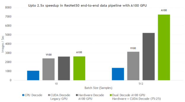
For more information, see Loading Data Fast with DALI and the New Hardware JPEG Decoder in NVIDIA A100 GPUs.
Optical flow accelerator
Optical flow and stereo disparity are two fundamental and related ways of analyzing images in computer vision. Optical flow measures the apparent motion of points between two images, while stereo disparity measures the (inverse) depth of objects from a system of two parallel calibrated cameras. This is demonstrated in Figure 8.
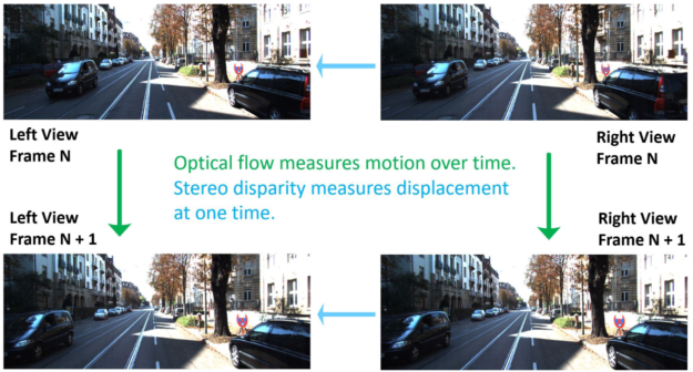
Optical flow and stereo disparity are used in computer vision tasks across a broad range of applications, including automotive and robotic navigation, movie production, video analysis and understanding, and augmented and virtual reality.
The measurement of optical flow and stereo disparity have been studied for decades, but despite great improvements in the state of the art, they remain challenging problems, especially to obtain real-time, dense data at the pixel rates of modern cameras, which routinely exceed 50 Mpixels/second and can easily reach 10 times that.
A100 includes a new improved optical flow engine that offers higher accuracy, per-pixel flow vectors, and region of interest. The module supports both optical flow and stereo disparity estimation at up to 300 fps at 4K. This hardware accelerator, which is independent of CUDA cores, calculates optical flow vectors between a given frame pair at high accuracy and high performance. Quality and performance can be tuned through parameter selection.
The optical flow hardware can be programmed using the NVIDIA Optical Flow SDK and is also accessible through DALI and OpenCV, a popular, open-source, computer vision library with tracking algorithms that can leverage optical flow hardware on NVIDIA GPUs to compute motion vectors.
Applications already leveraging the Optical Flow SDK get higher performance and higher accuracy on A100 with an upcoming driver update. APIs to take advantage of new features like region of interest and per-pixel flow vectors will be available in an upcoming release of the Optical Flow SDK.
Conclusion
The new A100 GPU is packed with new capabilities for computer vision workloads:
- Dedicated hardware for JPEG and video decoders to speed up the data input pipeline
- A new generation of hardware for optical flow acceleration
- New Tensor Core instructions to speed up FP32 data processing
- Improved throughput for FP16
- Multi-instance GPU that allows for better GPU sharing and isolation of workloads
All these A100 GPU capabilities are supported by NVIDIA NGC containers from versions 20.06, CUDA 11, and the upcoming releases of NVIDIA DALI and the Optical Flow SDK.
