AI applications are powered by machine learning models that are trained to predict outcomes accurately based on input data such as images, text, or audio. Training a machine learning model from scratch requires vast amounts of data and a considerable amount of human expertise, often making the process too expensive and time-consuming for most organizations.
Transfer learning is the happy medium between building a custom model from scratch and choosing an off-the-shelf commercial model to integrate into an ML application. With transfer learning, you can select a pretrained model that’s related to your solution and retrain it on data reflecting your specific use case. Transfer learning strikes the right balance between the custom-everything approach (often too expensive) and an off-the-shelf approach (often too rigid) and enables you to build tailored solutions with fewer resources.
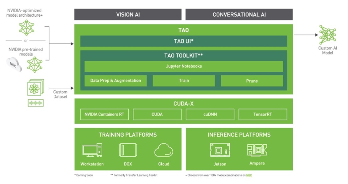
The NVIDIA TAO Toolkit enables you to apply transfer learning to pretrained models and create custom, production-ready models without the complexity of AI frameworks. To train these models, high-quality data is a must. While TAO focuses on the model-centric steps of the development process, Innotescus focuses on the data-centric steps.
Innotescus is a web-based platform for annotating, analyzing, and curating robust, unbiased datasets for computer vision–based machine learning. Innotescus helps teams scale operations without sacrificing quality. The platform includes automated and assisted annotation for both images and videos, consensus and review features for QA processes, and interactive analytics for proactive dataset analysis and balancing. Together, Innotescus and the TAO toolkit make it cost effective for organizations to apply transfer learning successfully in custom applications, arriving at high performing solutions in little time.
In this post, we address the challenges of building a robust object detection model by integrating the NVIDIA TAO Toolkit with Innotescus. This solution alleviates several common pain points that businesses encounter when building and deploying commercial solutions.
YOLO object detection model
Your goal in this project is to apply transfer learning to the YOLO object detection model in the TAO toolkit using data curated on Innotescus.
Object detection is the ability to localize and classify objects with a bounding box in an image or video. It is the most widely used application of computer vision technology. Object detection solves many complex, real-world challenges, such as the following:
- Context and scene understanding
- Automating solutions for smart retail
- Autonomous driving
- Precision agriculture
Why should you use YOLO for this model? Traditionally, deep learning–based object detectors operate through a two-stage process. In the first stage, the model identifies regions of interest in an image. In the second stage, each of these regions are classified.
Typically, many regions are sent to the classification stage, and because classification is an expensive operation, two-stage object detectors are extremely slow. YOLO stands for “You only look once.” As the name suggests, YOLO can localize and classify simultaneously, leading to highly accurate real-time performance, which is essential for most deployable solutions. In April 2020, the fourth iteration of YOLO was published. It has been tested on a multitude of applications and industries and has proven to be robust.
Figure 1 shows the general pipeline for training object detection models. For each step of this more traditional development pipeline, we discuss the typical challenges that people encounter and how the combination of TAO and Innotescus solves these problems.

Before you begin, install the TAO toolkit and authenticate your instance of the Innotescus API.
Installing TAO Toolkit
The TAO toolkit can be run as a CLI or in a Jupyter notebook. It’s only compatible with Python3 (3.6.9 and 3.7), so first install the prerequisites.
- On Linux, check the post-installation steps to ensure that Docker can be run without
sudo. - Install nvidia-container-toolkit.
- Create an NGC account and generate an API key for authentication.
- Log in to the NGC Docker registry by running the command
docker login nvcr.ioand enter your credentials for authentication.
After the prerequisites are installed, install the TAO toolkit. NVIDIA recommends installing the package in a virtual environment using virtualenvwrapper. To install the TAO launcher Python package, run the following commands:
pip3 install nvidia-pyindex
pip3 install nvidia-tao
Check whether you’ve gone through the installation correctly by running tao --help.
Accessing the Innotescus API
Innotescus is accessible as a web-based application, but you’ll also use its API to demonstrate how to accomplish the same tasks programmatically. To begin, install the Innotescus library.
pip install innotescus
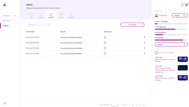
Next, authenticate the API instance using the client_id and client_secret values retrieved from the platform.
from innotescus import client_factory
client = client_factory(client_id=’client_id’, client_secret=’client_secret’)
Now you’re ready to interact with the platform through the API, which you’ll do as you walk through each step of the pipeline that follows.
Data collection
You need data to train the model. Though it’s often overlooked, data collection is arguably the most important step in the development process. While collecting data, you should ask yourself a few questions:
- Is the training data adequately representative of each object of interest?
- Are you accounting for all the scenarios in which you expect the model to be deployed?
- Do you have enough data to train the model?
You can’t always answer these questions completely but having a well-rounded game plan for data collection helps you avoid issues during subsequent steps in the development process. Data collection is a time-consuming and expensive process. Because the models provided by TAO are pretrained, the data requirements for retraining are much smaller, saving organizations significant resources in this phase.
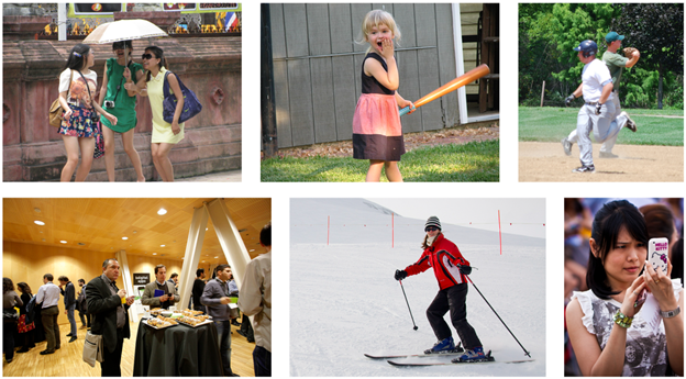
For this experiment, you use images and annotations from the MS COCO Validation 2017 dataset. This dataset has 5,000 images with 80 different classes, but you only use the 2,685 images containing at least one person.
%matplotlib inline
from pycocotools.coco import COCO
import matplotlib.pyplot as plt

dataDir=’Your Data Directory’
dataType=’val2017’
annFile=’{}/annotations/instances_{}.json’.format(dataDir,dataType)

coco=COCO(annFile)

catIds = coco.getCatIds(catNms=[‘person’]) # only using ‘person’ category
imgIds = coco.getImgIds(catIds=catIds)

for num_imgs in len(imgIds):
	img = coco.loadImgs(imgIds[num_imgs])[0]
	I = io.imread(img[‘coco_url’])
With the authenticated instance of the Innotescus client, begin setting up a project and uploading the human-focused dataset.
#create a new project
client.create_project(project_name)
#upload data to the new project
client.upload_data(project_name, dataset_name, file_paths, data_type, storage_type)
data_type: The type of data this dataset holds. Accepted values:DataType.IMAGEDataType.VIDEO
storage_type: The source of the data. Accepted values:StorageType.FILE_SYSTEMStorageType.URL
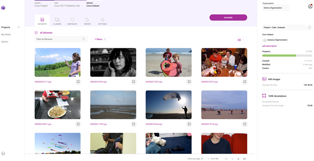
This dataset is now accessible through the Innotescus user interface.
Data curation
Now that you have your initial dataset, begin curating it to ensure a well-balanced dataset. Studies have repeatedly shown that this phase of the process takes around 80% of the time spent on a machine learning project.
Using TAO and Innotescus, we highlight techniques like pre-annotation and review that save time during this step without sacrificing dataset size or quality.
Pre-annotation
Pre-annotation enables you to use model-generated annotations to remove a significant amount of the time and manual effort necessary to label the subset of 2,685 images accurately. You use YOLOv4—the same model that you’re retraining—to generate pre-annotations for the annotators to refine.
Because pre-annotation saves you so much time on the easier components of the annotation task, you can focus your attention on the harder examples that the model can’t yet handle.
YOLOv4 is included in the TAO toolkit and supports k-means clustering, training, evaluation, inference, pruning, and exporting. To use the model, you must first create a YOLOv4 spec file, which has the following major components:
yolov4_configtraining_configeval_confignms_configaugmentation_configdataset_config
The spec file is a protobuf text (prototxt) message, and each of its fields can be either a basic data type or a nested message.
Next, download the model with pretrained weights. The TAO Toolkit Docker container provides access to a repository of pretrained models that serve as a great starting point when training deep neural networks. Because these models are hosted on the NGC catalog, you must first download and install the NGC CLI. For more information, see the NGC documentation.
After you’ve installed the CLI, you can see the list of pretrained computer vision models on the NGC repo, and download pretrained models.
ngc registry model list nvidia/tao/pretrained_*
ngc registry model download-version /path/to/model_on_NGC_repo/ -dest /path/to/model_download_dir/
With the model downloaded and spec file updated, you can now generate pre-annotations by running the inference subtask.
tao yolo_v4 inference [-h] -i /path/to/imgFolder/ -l /path/to/annotatedOutput/ -e /path/to/specFile.txt -m /path/to/model/ -k $KEY
The output of the inference subtask is a series of annotations in the KITTI format, saved in the specified output directory. Figure 6 shows two examples of these annotations:
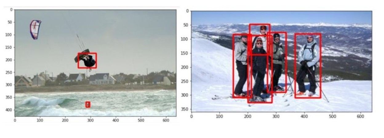
Upload the preannotations into the Innotescus platform manually through the web-based user interface or using the API. Because the KITTI format is one of the many accepted by Innotescus, no preprocessing is needed.
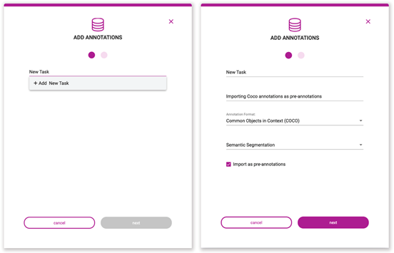
#upload pre-annotations generated by YOLOv4
Response = client.upload_annotations(project_name, dataset_name, task_type, data_type, annotation_format, file_paths, task_name, task_description, overwrite_existing_annotations, pre_annotate)
project_name: The name of the project containing the affected dataset and task.dataset_name: The name of the dataset to which these annotations are to be applied.task_type: The type of annotation task being created with these annotations. Accepted values from theTaskTypeclass:CLASSIFICATIONOBJECT_DETECTIONSEGMENTATIONINSTANCE_SEGMENTATION
data_type: The type of data to which the annotations correspond. Accepted values:DataType.IMAGEDataType.VIDEO
annotation_format: The format in which these annotations are stored. Accepted values from theAnnotationFormatclass:COCOKITTIMASKS_PER_CLASSPASCALCSVMASKS_SEMANTIC
MASKS_INSTANCEINNOTESCUS_JSONYOLO_DARKNETYOLO_KERAS
file_paths: A list of file paths containing the annotation files to upload.task_name: The name of the task to which these annotations belong; if the task does not exist, it is created and populated with these annotations.task_description: A description of the task being created, if the task does not exist yet.overwrite_existing_annotations: If the task already exists, this flag allows you to overwrite existing annotations.pre_annotate: Allows you to import annotations as pre-annotations.With the pre-annotations imported to the platform and a significant amount of the initial annotation work saved, move into Innotescus to further correct, refine, and analyze the data.
Review and correction
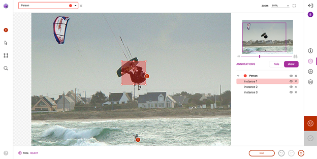
With the pre-annotations successfully imported, head over to the platform to perform review and correction of the pre-annotations. While the pretrained model saves a significant amount of annotation time, it’s still not perfect and needs a bit of human in the loop interaction to ensure high-quality training data. Figure 8 shows an example of a typical correction that you might make.
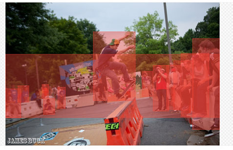
Beyond a first pass at fixing and submitting pre-annotations, Innotescus enables a more focused sampling of images and annotations for multistage review. This enables large teams to ensure high quality throughout the dataset systematically and efficiently.
Exploratory data analysis
Exploratory data analysis, or EDA, is the process of investigating and visualizing datasets from multiple statistical angles to get a holistic understanding of the underlying patterns, anomalies, and biases present in the data. It is an effective and necessary step to take before thoughtfully addressing the statistical imbalances your dataset contains.
Innotescus provides precalculated metrics for understanding class, color, spatial, and complexity distributions for both data and annotations, and enables you to add your own layer of information in image and annotation metadata to incorporate application-specific information into the analytics.
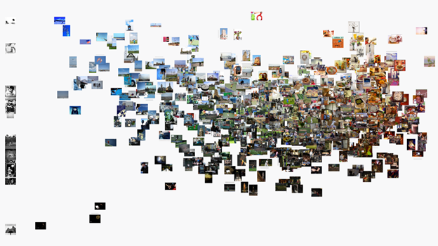
Here’s how you can use the Innotescus’s dive visualization to understand some of the patterns and biases present in the dataset. The following scatter plot shows the distribution of image entropy, which is the average information or degree of randomness in an image, within the dataset along the x-axis. You can see a clear pattern, but you can also spot anomalies like images with low entropy or information content.
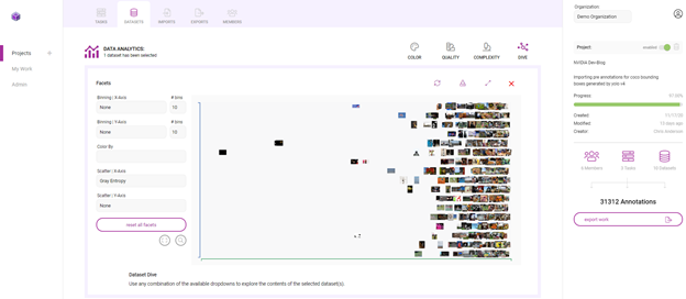
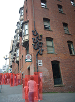

Outliers like these raise questions of how to handle anomalies within a dataset. Recognizing anomalies enables you to ask some crucial questions:
- Do you expect the model, when deployed, to encounter low-entropy input?
- If so, do you need more such examples in the training dataset?
- If not, are these examples going to be detrimental for training, and should they be removed from the training dataset?
In another example, look at each annotation’s area, relative to the image that it’s in.
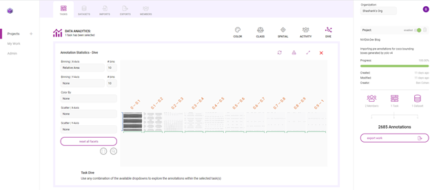


In Figure 13, the two images show the variation in annotation sizes within the dataset. While some annotations capture people that take up lots of the image, most show people far away from the camera.
Here, a large percentage of annotations are between 0 and 10% of their respective image sizes. This means that the dataset is biased towards small objects, or people that are far from the camera. Do you then need more examples in the training data that have larger annotations to represent people closer to the camera? Understanding the data distribution in this way helps you to begin thinking about the plan for data augmentation.
With Innotescus, EDA is made intuitive. It provides you with the information that you need to make powerful augmentations to your dataset and eliminate bias early in the development process.
Cluster rebalancing with dataset augmentation
The idea behind augmentation for cluster rebalancing is powerful. This technique showed a 21% boost in performance in the recent datacentric AI competition hosted by Andrew Ng and DeepLearning.AI.
You generate an N-dimensional feature vector for each data point (each bounding box annotation), and cluster all data points in higher dimensional space. When you cluster objects with similar features, you augment the dataset such that each cluster has equal representation.
We chose to use [red channel mean, green channel mean, blue channel mean, gray image std, gray image entropy, relative area] as the N-dimensional feature vector. These metrics were exported from Innotescus, which automatically calculated them. You could also use the embeddings generated by the pretrained model to populate the feature vector, which would arguably be more robust.
You use k-means clustering with k=4 as the clustering algorithm and UMAP for reducing the dimensions to two for visualization. The following code example generates the graph that shows the UMAP plot, color-coded with these four clusters.
import umap
from sklearn.decomposition import PCA
from sklearn.cluster import KMeans

# k-means on the feature vector
kmeans = KMeans(n_clusters=4, random_state=0).fit(featureVector)

# UMAP for dim reduction and visualization
fit = umap.UMAP(n_neighbors=5,
		min_dist=0.2,
		n_components=2,
		metric=’manhattan’)

u = fit.fit_transform(featureVector)

# Plot UMAP components
plt.scatter(u[:,0], u[:,1], c=(kmeans.labels_))
plt.title(‘UMAP embedding of kmeans colours’)
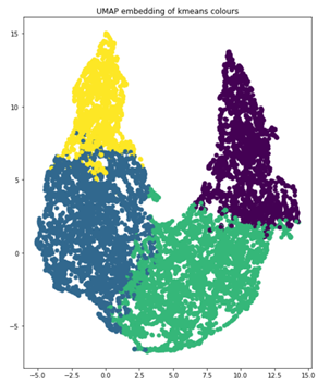
When you look at the number of objects in each cluster, you can clearly see the imbalance, which informs how you should augment the data for retraining. The four clusters represent 854, 1523, 1481 and 830 images, respectively. Where an image has objects in more than one cluster, group that image in the cluster with most of its objects for augmentation.
clusters = {}

for file, cluster in zip(filename, kmeans.labels_):
	if cluster not in clusters.keys():
		clusters[cluster] = []
		clusters[cluster].append(file)
	else:
		clusters[cluster].append(file)

for numCls in range(0, len(clusters)):
	print(‘Cluster {}: {} objects, {} images’.format(numCls+1, len(clusters[numCls]), len(list(set(clusters[numCls])))))
Output:
Cluster 1: 2234 objects, 854 images
Cluster 2: 3490 objects, 1523 images
Cluster 3: 3629 objects, 1481 images
Cluster 4: 1588 objects, 830 images
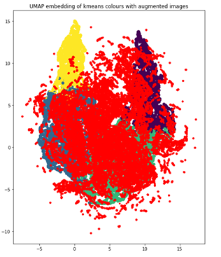
With the clusters well defined, you use the imgaug Python library to introduce augmentation techniques to enhance the training data: translation, image brightness adjustment, and scale augmentation. You augment such that each cluster contains 2,000 images for a total of 8,000. As you augment images, imgaug ensures that the annotation coordinates are altered appropriately as well.
import imgaug as ia
import imgaug.augmenters as iaa

# augment images
seq = iaa.Sequential([
	iaa.Multiply([1.1, 1.5]), # change brightness, doesn’t affect BBs
	iaa.Affine(
		translate_px={“x”:60, “y”:60},
		scale=(0.5, 0.8)
	) # translate by 60px on x/y axes & scale to 50-80%, includes BBs
])

# augment BBs and images
image_aug, bbs_aug = seq(image=I, bounding_boxes=boundingBoxes)
Using the same UMAP visualization technique, with augmented data points now in red, you see that the dataset is now much more balanced, as it more closely resembles a Gaussian distribution.
Model training
With the well-balanced, high-quality training data, the final step is to train the model.
YOLOv4 retraining on TAO Toolkit
To start retraining the model, first ensure that the spec file contains the classes of interest, as well as the correct directory paths for the pretrained model and training data. Change the training parameters in the training_config section. Reserve 30% of the augmented dataset as a test dataset to compare the performance of the pretrained model and the performance of the retrained model.
ttraining_config {
	batch_size_per_gpu: 8
	num_epochs: 80
	enable_qat: false
	checkpoint_interval: 10
	learning_rate {
		soft_start_cosine_annealing_schedule {
			min_learning_rate: 1e-7
			max_learning_rate: 1e-4
			soft_start: 0.3
		}
	}
	regularizer {
		type: L1
		weight: 3e-5
	}
	optimizer {
		adam {
			epsilon: 1e-7
			beta1: 0.9
			beta2: 0.999
			amsgrad: false
		}
	}
	pretrain_model_path: “path/to/model/model.hdf5”
}
Run the training command.
tao yolo_v4 train -e /path/to/specFile.txt -r /path/to/result -k $KEY
Results
As you can see, you achieved a 14.93% improvement in the mean average precision, a 21.37% boost from the mAP of the pretrained model:
| Model | mAP50 |
| Yolov4 pretrained model | 69.86% |
| Yolov4 retrained model with cluster-rebalanced augmentation | 84.79% |
Summary
Using NVIDIA TAO Toolkit for pre-annotation and model training and Innotescus for data refinement, analysis, and curation, you improved YOLOv4’s mean average precision on the person class by a substantial amount: over 20%. Not only did you improve the performance on a selected class, you used less time and data than you would have without significant benefits of transfer learning.
Transfer learning is a great way to produce high-performing, application-specific models in settings with constrained resources. Using tools like the TAO toolkit and Innotescus makes it feasible for teams of all sizes and backgrounds.
Try it for yourself
Interested in using Innotescus to enhance and refine your own dataset? Sign up for a free trial. Get started with the TAO toolkit for your AI model training by downloading the sample resources.
