GPU-driven rendering has long been a major goal for many game applications. It enables better scalability for handling large virtual scenes and reduces cases where the CPU could bottleneck a game’s performance.
Short of running the game’s logic on the GPU, I see the pinnacle of GPU-driven rendering as a scenario in which the CPU sends the GPU only the new frame’s camera information, while the GPU takes care of the rest, all the way down to the final pixels presented on-screen.
The Direct3D 12 (D3D12) API has taken several steps in this direction, including such features as ExecuteIndirect, Unbounded Resource Arrays, and ResourceDescriptorHeap.
Work graphs are another feature that I’m excited to discuss. Work graphs provide a programming paradigm that enables the GPU to generate work for itself on the fly. This offers a solution to some well-known game engine problems, and opens the path to new creative ideas.
This post introduces high-level concepts of work graphs: the structure, launch modes, and data flow. I explain how a work graph can be written in HLSL, as well as the steps involved in launching a work graph from the CPU. To get the most from this post, you should have some familiarity with:
- The D3D12 API
- Writing and compilation of compute shaders
ExecuteIndirectand ray-tracing APIs
Note that work graphs are supported on NVIDIA Ampere architecture and NVIDIA Ada Lovelace architecture. An NVIDIA display driver with version 551.76 or later is also required, and can be found through NVIDIA Driver Downloads.
Work graphs overview
Shader Model 6.8 for D3D12, among many other features, marks the official release of work graphs. The term ‘graph’ in the name holds up well to its definition: a collection of nodes connected by edges. In work graphs, nodes perform tasks (“work”) and pass data to other nodes across the graph edges.
But what is this work that a node executes? Is it a command such as a Dispatch call? A single thread running a certain shader? Or perhaps a group of threads running the same shader?
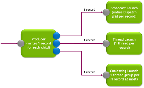
The answer is, all of the above. Each node has a shader that is launched in a certain configuration of the programmer’s choice. This configuration, or launch mode, can be a full dispatch grid (broadcast launch) or compute threads run either independently of each other (thread launch) or potentially collectively (coalescing launch). Note that Thread Launch work can be gathered to run in a wave where possible, but each thread will still have its inputs independent of other threads.
A connection to another node is realized by choosing the target node and passing data to it. This resembles what is typically known as continuation in graph terminology. The target node receives the data and runs outside its caller’s context. There is no call stack in this system, just data cascading from the top to the bottom of the graph.
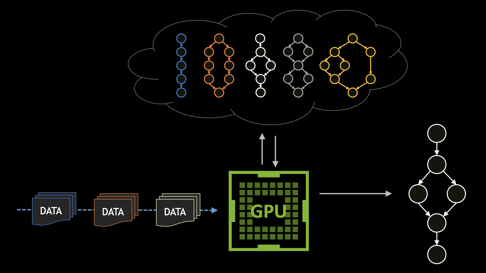
Units of data, called records, drive the entire execution of the work graph. To launch a node, a record must be written for it. The node’s shader is then launched in the chosen launch mode, and consumes that record as input. The record is a packed structure of data filled by the producer. The producer could be the CPU’s command DispatchGraph, or any node in the work graph. A node consuming the record could be thought of as a child of the producer node.
Work graphs new functionality
D3D12 already exposes functionality to aid in GPU-driven rendering, as mentioned previously. This section highlights the new functionality introduced by work graphs, compared to existing functionality.
Dynamic shader selection
Each node in the work graph can choose which of its children to run. The decision is driven by the producer’s shader code itself. This enables decisions to be determined by information generated by the GPU in a previous node or workload.
On the other hand, ExecuteIndirect is confined to work under the state it was launched with, most notably the shader specified by the pipeline state object. An application that needs to launch different shaders depending on GPU-side data has no choice but to issue a series of SetPipelineState and ExecuteIndirect calls, or rely on inefficient uber shaders to cover only some of the potential possibilities.
Implicit micro-dependency model
Rendering a frame involves executing several major passes, such as depth, geometry, or lighting passes. Within each pass, data is processed in parallel, where each unit of data goes through several sequential operations. Resource barriers are usually placed between the operations to ensure data processing is completed by the previous operation before moving to the next.
A work graph expresses this dependency implicitly by producer nodes passing records to children nodes. Children node shaders will only run when the producer has completed writing the record, implying that the data is fully ready for consumption by the child. Note that the scope of work graph producer-consumer dependencies are on the data record scope, whereas a resource barrier operates on all accesses to a resource.
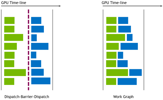
The work graph dependency model is fine-grained compared to barriers. This can translate to better occupancy on the GPU, as dependent work can launch earlier instead of waiting for a barrier to finish. Records can immediately pass from the producer to the consumer node and need not be fully flushed across algorithm steps as is the case for Dispatch-ResourceBarrier sequences.
Figure 2 illustrates how the workloads are executed in each case. On the left, two Dispatch calls separated by a ResourceBarrier. Each row represents a producer thread-group (green) and its consumer thread-group (blue). On the right, the same workloads run with a work graph.
Writing work graphs in HLSL
Similar to ray-tracing shaders, work graphs are written as a library of compute shaders. A single HLSL file may contain code for all the nodes in the graph. But it’s also possible to construct the graph from different sources and link those at once, or even gradually during run-time.
The following HLSL code snippet demonstrates a very simple work graph made of two nodes: a producer and a consumer node.
struct RecordData { int myData; };

[Shader("node")]
[NodeLaunch("thread")]
[NodeIsProgramEntry]
void MyGraphRoot(
    [MaxRecords(1)] NodeOutput<RecordData> MyChildNode)
{
    ThreadNodeOutputRecords<RecordData> childNodeRecord =
   	 MyChildNode.GetThreadNodeOutputRecords(1);
    childNodeRecord.Get().myData = 123456;
    childNodeRecord.OutputComplete();
}

[Shader("node")]
[NodeLaunch("broadcasting")]
[NodeDispatchGrid(1, 1, 1)]
[numthreads(8, 8, 1)]
void MyChildNode(
    DispatchNodeInputRecord<RecordData> inputData,
    uint2 dispatchThreadId : SV_DispatchThreadID)
{
    int myData = inputData.Get().myData;
}
This snippet shows how node shaders are basically regular compute shaders with some added declarations. Of note is the NodeLaunch attribute, which specifies the launch mode for that node. The root node in the graph (signified by the NodeIsProgramEntry attribute) is a thread launch node. Thus, for every input record, there will be a compute shader thread to process it. The root input records originate from the DispatchGraph call in the command list.
The shader function signature includes a parameter MyChildNode of type NodeOutput<RecordData>. This parameter can be used to produce records going to MyChildNode node of the graph. In this way, the name of the parameter must match with the name of another node in the graph.
MyChildNode is a broadcasting launch node. This means that a single record pushed to such a node will cause a similar effect to a Dispatch call with a certain grid size, determined here by the attribute NodeDispatchGrid associated with the MyChildNode function signature.
For more details about the new syntax and declarations, see the HLSL syntax reference for work graphs.
CPU-side setup
Launching a work graph requires similar steps needed by other kinds of work in D3D12; specifically:
- Perform feature support check
- Compile shaders either offline or during runtime
- Load shader library and construct work graph state object
- Allocate backing memory
- Launch the graph
Feature support check
To ensure work graphs are supported on the target machine, it’s necessary to call CheckFeaturesSupport and inspect the WorkGraphsTier field of the D3D12_FEATURE_DATA_D3D12_OPTIONS_21 structure.
Compile shaders
A work graph requires compiling the HLSL source code against the lib_6_8 shader target. There are no specific requirements to pass to the compiler, other than the standard switches used by other shader types.
Load shader library
The binaries from the compiler must be loaded and a D3D12_STATE_OBJECT_DESC must be prepared with all the parts needed for the work graph. Quite a few pieces of information must be provided, including:
- The DXIL library to use (that is, the precompiled shader binary).
- The root signature(s) used by the work graph.
- Which nodes will make up the graph (all of them or a certain subset).
- Overrides to certain attributes already set in the shader library (if needed). These overrides can drive static values in the work graph using values determined at run-time.
Allocate backing memory
The graph also requires backing memory for use during its execution. After creating the state object, memory requirements for the graph must be queried and the allocation must be made before launching the graph. If the reported backing memory requirement has a minimum size different from the maximum size, it’s recommended to respect the maximum size to enable best performance of graph execution.
Launch the graph
This step is very similar to launching a compute shader. The command list must be in a good state, where objects like descriptor heaps, the root signature, root parameters, and descriptor tables are bound.
Launching the graph requires calling SetProgram on the command list first. This call specifies the graph to launch, its backing memory, and additional launch flags, if needed.
One important flag is D3D12_SET_WORK_GRAPH_FLAG_INITIALIZE. This flag must be passed the first time a work graph uses its backing memory. Subsequent launches can omit this flag as long as the backing memory was not used by something other than the graph itself.
Finally, call DispatchGraph. At this point, it’s possible to specify the input records for the root of the graph. Such records can be fed from CPU or GPU memory.
For reference, the sample code’s LoadWorkGraphPipelines and PopulateDeferredShadingWorkGraph functions show and explain each step in the entire CPU-side setup process.
Expressing algorithms with work graphs
It is important to understand how work graphs operate and what their capabilities and limitations are. With this understanding, you can take any algorithm and decide how to express it as a work graph in the most efficient manner.
Work graphs promote data flow and transformation operations. That is, independent data that must flow through a number of steps, transforming and potentially expanding along the way to the final result.
Considerations when working with this version of work graphs include the following:
- With the exception of the root input records, concrete numbers, or upper limits, must be specified for work size and potential expansions in the graph. For example, a broadcast launch node must either use a fixed dispatch grid size, or provide an upper limit for it. As a developer, you must be able to derive those numbers from the algorithm and the potential size of its inputs.
- A node may only take one input record type. Multiple input record types are not allowed. This means a single node cannot be a “join” target of different producers. While it is possible to work around this and manually implement such joins, I suggest avoiding it. Such joins imply that data records linger in the graph’s execution memory until all input records become ready and the join target can launch. Note that coalescing nodes are not suitable to solve this, as their launch condition doesn’t guarantee the number of input records, and may launch with a lower number.
- A graph may not contain any loops, with one exception: a node can loop to itself.
- The graph may not go deeper than 32 nodes. A node’s maximum number of self-loops is also counted against this number.
- Nodes cannot yet produce draw calls, but keep in mind that
TraceRayInlinecan be used. - Resources cannot transition to different states during the execution of the work graph.
Conclusion
Work graphs in the Direct3D 12 API help to solve some well-known problems, and enable new creative ideas. In this post, I explained the different launch nodes and how to pass data through records. I also discussed HLSL code for a work graph, as well as the steps involved in launching a work graph from the CPU. Finally, I covered the mental model behind this feature, and how best to map GPU algorithms to it, given certain limitations on this version of work graphs. To see all the details necessary to build and run work graphs, visit NVIDIAGameWorks/donut_examples on GitHub.
To read more about work graphs, including advanced topics and a case study, see Work Graphs in Direct3D 12: A Case Study of Deferred Shading.