Work Graphs in Direct3D 12: A Case Study of Deferred Shading

When it comes to game application performance, GPU-driven rendering enables better scalability for handling large virtual scenes. Direct3D 12 (D3D12) introduces work graphs as a programming paradigm that enables the GPU to generate work for itself on the fly. For an introduction to work graphs, see Advancing GPU-Driven Rendering with Work Graphs in Direct3D 12.

This post features a Direct3D 12 work graphs case study. I explain how the common deferred shading rendering algorithm can benefit from work graphs’ efficient shader code selection and execution. Then, from this case study, I explore more advanced topics, learnings, and recommendations for work graphs.

Work graphs selective shader code execution

Compared to ExecuteIndirect, work graphs in the Direct3D 12 (D3D12) API have a unique capability to dynamically choose and launch shaders on a micro-level. For example, consider an operation that partitions the screen into tiles. For each tile, a certain operation must be performed depending on the contents of that tile. Suppose there are 10 possibilities for each tile. You can accomplish this using three different approaches:

1. Use an uber shader with a large switch/case block that contains code for all possibilities.
2. Issue full-screen Dispatch calls that run a shader specialized for each of the possibilities. The shader first determines whether the tile is about to process matches with the shader. If not, the shader exits immediately.
3. Start with a pass that classifies the tiles and counts how many tiles there are for each possibility. Then use ExecuteIndirect to enable the GPU to adjust the grid size for each of the dispatches.

Each of these approaches comes with its drawbacks. For the first approach, an uber shader often leads to waste in the register file, caused by variables that must be kept alive even if not used for a particular execution path, thus reducing occupancy. There is also some cost due to the branching in the switch/case block.

The second approach suffers from launching a wasteful number of compute warps in order to cover all possibilities. The third approach sounds most efficient, but introduces a classification pass not present in the first two approaches.

Work graphs offer a more elegant solution. The following case study will show how, including recommendations and useful tools for debugging. 

Multi-BRDF deferred shading case study

Deferred shading has been a very common technique for managing lighting and material interactions in a game engine. Typically, meshes in the scene are rasterized into a fat G-buffer that stores shading parameters for each pixel (normal, albedo, and roughness, for example). Then a follow-up lighting pass takes the information from the G-buffer and applies lighting to the contents to produce a lit pixel and stores it in a color buffer, usually in HDR format.

The lighting pass itself is usually accompanied by some acceleration structure that enables the shader to consider only lights that affect the pixel underneath, instead of checking against all light sources in the scene.

This works fine as long as all materials in the scene use the same Bidirectional Reflectance Distribution Function (BRDF), which can be artistically limiting. To support more than one BRDF (for example, clear-coat, eye, or hair), an additional parameter can be added to the G-buffer to signify the BRDF for each pixel. In addition, the lighting pass must use a switch/case block on that BRDF value so it knows how to compute the material-light interaction. Does this sound familiar? 

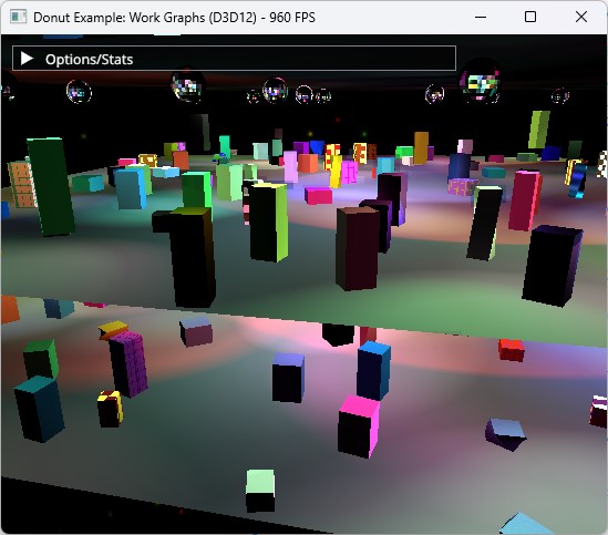
I have built a sample around this use case to explore how work graphs could help. The fully documented sample code implements a multi-BRDF deferred shading renderer. Available through NVIDIAGameWorks/donut_examples on GitHub, it showcases two approaches: uber shaders and work graphs. 

This sample uses a slim G-buffer layout that stores only the normal and material IDs instead of all material parameters. This makes sense for multi-BRDF materials, as each BRDF could have a different set of parameters to represent a material. During shading, the material type is used to determine the logic for pulling the material parameters and evaluating the material-light interaction.

The scene is made up of multiple dance floors. Each floor is populated by an animated crowd of cuboids. The ceiling is populated with reflective balls that cast moving lights on each floor. Numerous colored moving spotlights also light the scene. 

This scene is fully procedurally generated and animated. Several controls manage scene complexity (number of meshes, lights, and materials). Materials can use one of several types (or BRDFs) that render in a certain way (Lambert, Phong, Metallic, or Velvet, for example).

Take your time tweaking the code and trying different scene parameters to see how these changes affect performance.

The standard deferred shading compute pass is done using two compute dispatches:

1. Tiled light culling: The screen is divided into tiles that are 8×4 pixels each. For each tile, all lights affecting that tile are collected and stored in a buffer.
2. Deferred shading using an uber shader: Each tile is processed again, this time using the lights collected by the tile. All materials found in the tile are evaluated in an uber shader.

Most importantly, this sample implements the same deferred shading pass using work graphs.

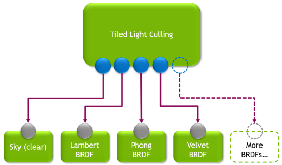
The work graph technique completely replaces the two steps mentioned previously. Instead, the graph uses broadcasting launch nodes to replicate the same concept of tiled light culling. The root node of the graph is executed for each screen tile. The node culls lights for the tile, and stores the results in a record to be sent to the next step of the graph.

The root node can target an array of outputs, where each output is specialized for a certain BRDF (or a screen clear). The culled lights list is placed in a record that’s sent to the correct node in the graph that can handle the type of material in the tile. In the case of a tile containing multiple different BRDFs, the root node spawns multiple records to cover the same tile using all the proper nodes.

Performance

On a GeForce RTX 4090 GPU, the work graph lights the scene at 1920 x 1080 within 0.8 ms to 0.95 ms, whereas the uber shader dispatch technique takes 0.98 ms. Multiple factors lead to these results, as detailed below.

1. Work graph execution is not free. There is a cost associated with managing the graph’s records and scheduling work. This cost eats some of the gains the work graphs achieved. 
2. Lighting performance using work graphs responds better to screen content. When the screen contains a lot of Sky tiles, the lighting pass finishes faster. In this case, the performance difference between a screen full of meshes and a screen half-full of meshes (depending on the view) is about 0.2 ms. The uber shader performance does not respond as well to screen content. It demonstrates mostly stable time regardless of view.
3. Node shaders in the work graph are specialized to handle one BRDF each, whereas the uber shader must handle all possible BRDFs. The node shaders thus have a better chance of compiler optimizations.
4. BRDF node shaders can launch as soon as the root node has classified the tile. The uber shader technique involves two dispatches separated by a resource barrier, which means the second dispatch can only launch after the first dispatch is fully complete.

These results portray one of the lessons I learned during my adventures with work graphs. That is, the performance gains must outweigh the overhead cost of work graph execution in order to see a net win in performance. The sample shows how the deferred shading pass can benefit from work graphs, even though this version of work graphs is limited to compute shaders only.

Content streaming game engines

This section explores how a renderer that uses work graphs could support large-scale game worlds. Consider an engine that enables artists to author material shaders. The concept of multi-BRDF simply becomes applicable on the material itself, where each material has a shader of its own that executes its unique computations—and even the BRDF altogether.

A problem can arise when materials are loaded gradually with the rest of the game’s content as the player is progressing or moving across different parts of the game world in a seamless manner. This is commonly referred to as content streaming. From a graphics programming perspective, it involves loading resources on the fly, including textures, meshes, and materials.

In the scheme of a single work graph handling all materials of the scene, how can the graph grow to handle more materials as the need arises during runtime?

A naive approach would be to fully rebuild the HLSL code of the graph and inject the new material’s shader code into it. Not only does this lead to a whole bunch of extremely slow string operations, but the cost of compilation could be too high to hide, resulting in strong stutters in gameplay. Avoid this approach.

A less naive approach is to completely recreate the graph, with the addition of precompiled DXIL libraries for the new materials. 

The ideal approach is to use the AddToStateObject API to support streaming scenarios in ray tracing applications. Work graphs make it easy to extend the nodes that could be targeted by any certain producer thanks to sparse node output arrays.

In this case, it would be possible to have the node responsible for material classification to declare its target outputs as a sparse output array. Each output of the array maps to a node representing a specific material shader, and those nodes are indexed by an integer value that can be chosen dynamically. Refer to the DirectX Specs to learn how to use this feature.

Recommendations

After spending some time with work graphs, I have collected a list of learnings and recommendations that should help make the process more fun, and reduce unhappy surprises.

• When designing or adapting existing algorithms to work graphs, understand the mental model of data being communicated from top to bottom, driving work that can potentially expand.
• Work graphs excel in their ability to execute different shaders according to different conditions. Avoid uber shader nodes. Instead, break such shaders down into individual, simpler, specialized node shaders. Such specialized shaders benefit from reduced register pressure and less chance of divergent execution.
• Aim for node shaders that do a considerable amount of work rather than a small set of operations. Otherwise, the cost of the work graph will be dominated by its execution overhead.
• Avoid UAV reads and writes to the same resource in the graph where possible. Such resources require the globallycoherent specifier to maintain correctness, but this specifier will also affect access speed considerably on such resources. Embrace communicating work data across nodes using records.
• For broadcast launch nodes, if the dispatch size can be determined statically, use NodeDispatchGrid attribute to specify the size instead of passing the grid size as an SV_DispatchGrid value in the input record. Remember that it is possible to override NodeDispatchGrid during work graph creation at runtime to adjust it according to certain runtime conditions like screen resolution and other quality settings.
• Try to keep the numbers specified in attributes like NodeMaxDispatchGrid and MaxRecords as tight as possible. Understand the broadcast/coalescing nature at the various nodes of the work graph, and use this understanding to determine good values for work size estimation. This should help reduce the backing memory size required by the graph.
• Consider marking node outputs with the MaxRecordsSharedWith attribute where possible. One obvious and common case is if a producer node thread will write one output record to only one of its children.
• Aim to complete outputting node records as early as possible in the shader and use OutputComplete to mark the completion. This gives a better chance for improved occupancy.
• Start simple and validate that each step works correctly before adding code to launch the next node. It’s easy to make mistakes, especially when requesting output records. Since work graphs are a new feature, debugging tools are not yet optimal.

Profiling and debugging tools

NVIDIA Nsight Graphics provides comprehensive support for profiling and debugging graphics applications. It exposes the rendering pipeline and visualizes your workloads, helping you identify and solve optimization needs. 

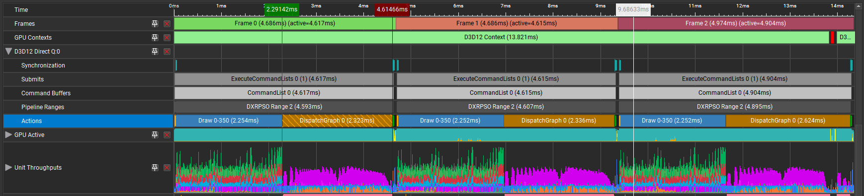
You can examine D3D12 work graphs in the Nsight Graphics Frame Debugger, which inspects GPU processes frame by frame. By capturing and replaying work graphs, the Frame Debugger can reveal API parameters, resource bindings, and the contents of memory buffers. 

The function DispatchGraph launches a work graph onto the GPU, and orchestrates how tasks are executed in a graph structure, enabling efficient parallelism and task dependency management. This function is plotted as a timeline event in Nsight Graphics GPU Trace, so you can view GPU performance metrics alongside it. 

Future directions

Many algorithms revolve around large amounts of independent data flowing through a series of steps, with expansions occurring at various steps. Algorithms processing hierarchical data stand to be great candidates for work graph implementations. For example, the process of taking a virtual scene, culling it to the visible area, processing and transforming meshes, all up to triangle rasterization. This process can be implemented well in a single work graph.

Although work graphs are currently limited to compute shaders, it is possible to build a specialized rasterizer in compute or even use inline ray tracing. However, this should not be necessary once work graphs add support for submitting triangles to the rasterizer.

Work graphs take a big step toward full GPU-driven frame processing. But it is not yet possible for one work graph to express the work of an entire frame (for example, culling, rasterizing a G-buffer, lighting then postprocessing). While a single work graph can represent multiple steps of the frame’s rendering, there are still some operations that cannot be done efficiently within a single work graph. Questions that arise when operating with such a wide scope include:

• How should resource states be managed during graph execution?
• How can triangles be submitted to the hardware rasterizer? Can further parts of the work graph run following triangle rasterization?
• How can multi-pass algorithms be represented (postprocessing chains, for example)?

Until these questions are resolved, the CPU will continue to play a primary role in frame sequencing. Yet more data-dependent passes can now be moved entirely to the GPU, freeing the CPU from tasks like having to manage scene culling and push commands for every visible entity. So, we are not yet at a point where the CPU can submit just one call to DispatchGraph to draw the entire frame, but this release of work graphs helps convert more parts of the frame to become GPU-driven, thus reducing the cases where the CPU would be the bottleneck for the application’s performance.

Conclusion

This post has explored a concrete use case that formulates an existing rendering algorithm to benefit from the capabilities of work graphs in Direct3D 12. I also discussed some advanced topics about work graphs, including performance considerations and operation under streaming game engines. And I explained support for work graphs in the latest release of NVIDIA Nsight Graphics. To see all the details necessary to build and run work graphs, visit NVIDIAGameWorks/donut_examples on GitHub. 

Acknowledgments

Thanks to Avinash Baliga and Robert Jensen from the NVIDIA Nsight Graphics team for contributing to this post.