Accelerating Product Development with Physics-Informed Neural Networks and NVIDIA Modulus

NVIDIA Modulus was previously known as NVIDIA SimNet.

Simulations have been widely used to model a variety of real-world problems in the science and engineering domains. Recent developments in AI and machine learning have led to the use of data to build surrogates for simulations, but the latest efforts have focused on the infusion of scientific laws in neural networks.

NVIDIA Modulus is an AI toolkit based on physics-informed neural networks (PINNs) that can be used to solve forward, inverse, and data assimilation problems. Engineers, scientists, students, and researchers who are looking to solve complex nonlinear physics problems with real-world applications can benefit from Modulus by using AI-driven physics simulations.

A success story of Modulus application today is in the automation of design optimization of manufacturing and environmental air control systems. These enable product designers to investigate the performance of any given design without a great deal of prior domain expertise. This application uses physics-informed neural networks (PINNs) in coupling detailed fluid dynamics solutions for 2D nozzle flows with commercial CAD software.

The effort was led by Michael Eidell, a senior engineer in the Modeling & Simulations Group at Kinetic Vision, a Cincinnati-based technology company that serves the Fortune 500. He focuses on finding insights for his clients quickly and relaying those findings in compelling ways to help the clients meet their complex product and system development needs with efficient concept-to-production solutions.

The major distinguishing factor that Michael’s team observed between Modulus and traditional computational physics tools is that it doesn’t rely upon a mesh to discretize the domain and its geometry module provides the flexibility to build parametric features, for example, edge radii. The scalability of the code on multiple GPUs was another factor that played a role in the Kinetic Vision team’s success in demonstrating Modulus as a viable product design tool.

Product design and optimization through simulation

As a company that has a large product design group, engineers at Kinetic Vision typically perform detailed computational physics assessments (for example, FEA, CFD) of design performance. This often consists of performing multiple design iterations, generating various computational meshes, and running a first principles solver. The run time and labor associated with such a process can be prohibitively expensive and time-intensive when a large number of design variables are considered. In some cases, a reduction in model fidelity may be appropriate. But for problems involving complex fluid dynamics, the full Navier-Stokes equations must be considered.

Michael and his team had previously explored the use of other commercial solvers for developing a simple fluid model of a 2D nozzle. However, they decided to use the Modulus platform due to multiple factors:

The team’s experience with GPUs in the machine learning realm was quite significant.
There is a strong desire within the company to explore the usage of GPUs in physics-based modeling to help accelerate the product design process and modeling and simulation work.
The Modulus API is Python-based, which makes it much easier to adopt and to begin prototyping on real world problems.

Modulus was perfectly aligned with the team’s experience and development goals.

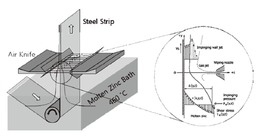
Michael’s team started building a 2D model of a 3D air-knife system that mimics the hot gas wiping systems employed during galvanization. The air knife is a subsonic gas nozzle that issues the gas out onto a nearby strip of steel, which has been bathed in molten zinc. The gas helps maintain a consistent zinc thickness on the steel strip, thereby galvanizing the steel (Figure 1).

An air knife system with steel strip and molten zinc bath — *Figure 1. Schematic diagram of a hot-dip galvanizing process with air knife.* Source: *A Noble Gas Wiping System to Prevent the Edge Overcoating in Continuous Hot-dip Galvanizing*

Getting started with Modulus

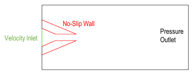
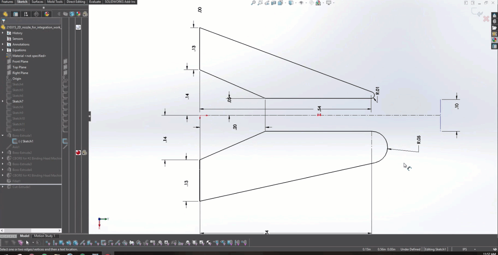
Using the Modulus geometry module, the subsonic gas nozzle was modeled as an inlet, a solid wall, and a pressure outlet to model the ambient environment (Figure 2).

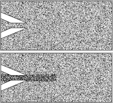
No-slip wall with velocity inlet and pressure outlet — *Figure 2. The Modulus domain of interest and boundary conditions employed during the training of the PINN*

The meshless approach employed within Modulus still requires the domain of interest to be sampled properly to help capture all salient flow features. You can visualize the geometry using tools such as Paraview after the problem has been set up.

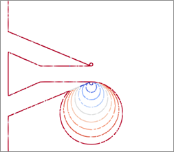
Figure 3 compares two different batch sampling approaches that can be taken in the 2D nozzle problem. The upper image shows a uniform sampling while the lower image includes a high-resolution region in the potential core of the jet flow where some of the largest velocity gradients may arise.

Exploring the Coanda effect as a method to control jet angle was of interest in this problem. Michael’s team explored it by adding in a radius to the trailing edges of the nozzle. The upper trailing edge of the nozzle had a fixed radius while the lower trailing edge of the nozzle was varied. Figure 4 shows a simple depiction of some discrete values of the radii explored on the lower trailing edge.

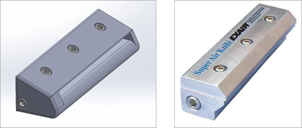
The final trained PINN was coupled to Solidworks to help demonstrate how a product designer could use the trained model in designing an air knife. The CAD model of a simple rectangular air knife was generated with existing products in mind.

*Figure 5. (left) A CAD model of the product being designed using Modulus trained results. (right) This product design was motivated by actual commercially available air knife products.*

Design optimization runs

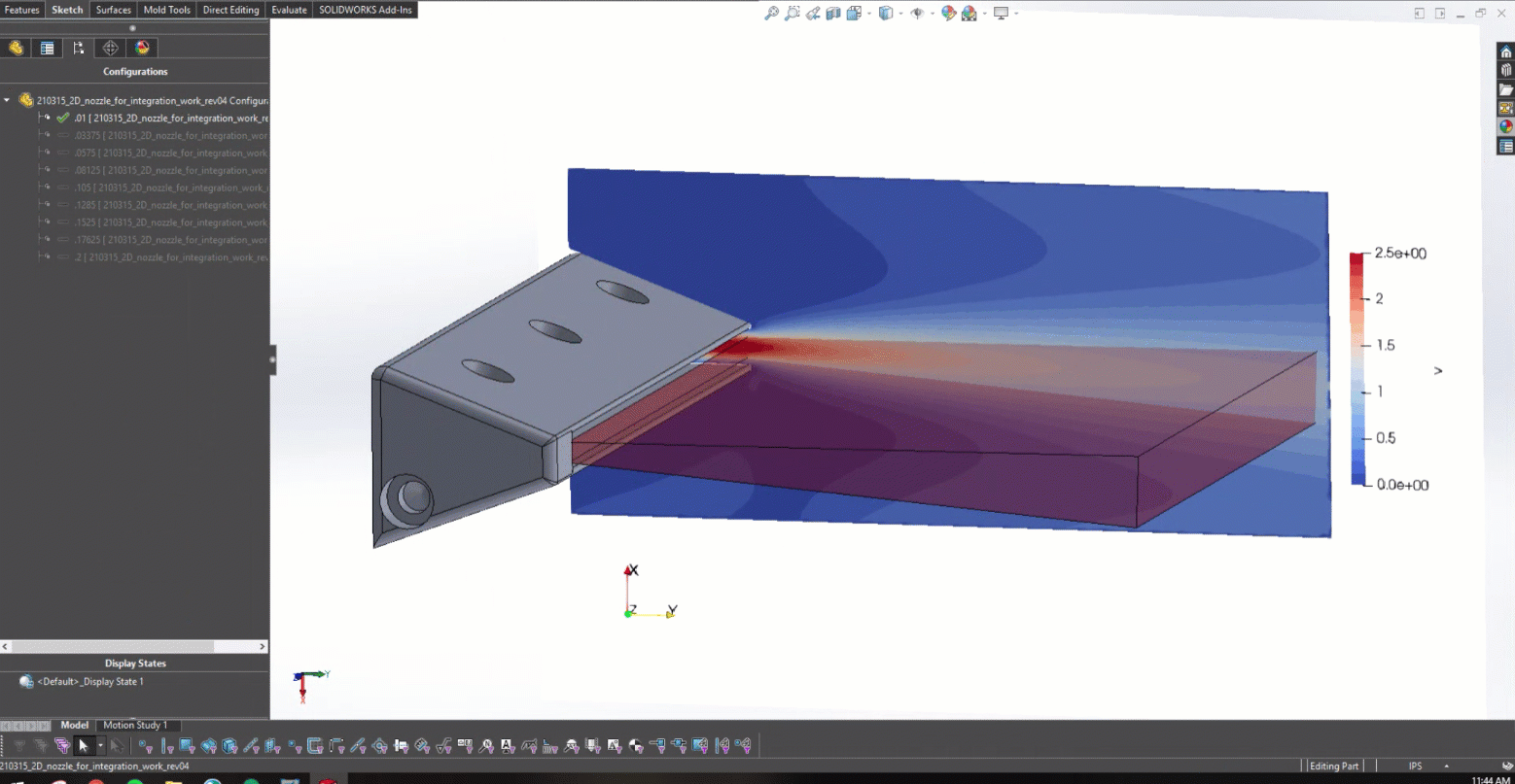
After training the PINN and developing the CAD model in Figure 5, it was possible to begin coupling with Solidworks. Figure 6 actually shows how changing the lower trailing edge radius provided the design with real-time feedback on what the resulting jet angle was.

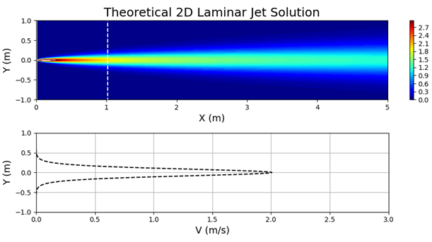
The animations show how changing the lower trailing edge radius provided the design with real-time feedback on what the resulting jet angle was.

*Figure 6. Animation of the changing lower trailing edge radius with the real-time feedback on the resulting jet angle*

In this work, the physics of the gas wiping process were reduced to that of a 2D isothermal, laminar jet. The equations governing such laminar jets are as follows:

$\label{eq:1} \frac{\partial u}{\partial x} + \frac{\partial v}{\partial y} = 0$

$\label{eq:2} u \frac{\partial u}{\partial x} + v \frac{\partial v}{\partial y} = \nu \frac{\partial^2 u}{\partial y^2}$

Equations 1 and 2 are the conservation of mass and momentum, respectively, for a 2D laminar jet where $u$ is the x-direction velocity, $v$ is the y-direction velocity, $\rho$ is the fluid density, and $\nu$ is the kinematic viscosity.

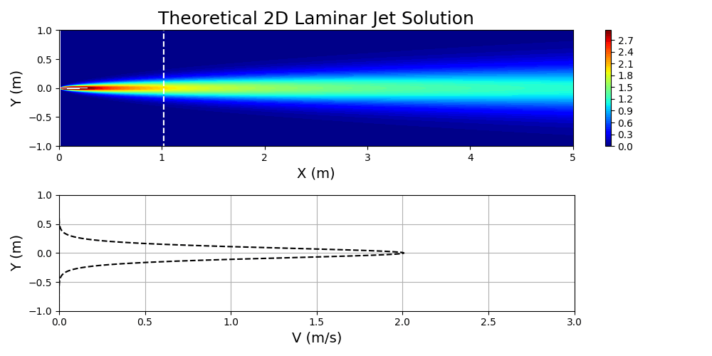
The solution to equations 1 and 2 can be carried out through similarity techniques that yield solutions of the following form:

$u=\left(\frac{3M^2}{32\rho^2\nu x}\right)^{1/3}\text{sech}^2\left[y\left(\frac{M}{48\rho\nu^2x^2}\right)^{1/3}\right]$

Figure 7 shows Equation 3 plotted for specified values of $M$ , $\nu$ , and $\rho$ .

Visualization of the theoretical 2D Laminar Jet Solution — *Figure 7. Visualization of the theoretical 2D laminar jet solution*

The fluid of interest in this problem was taken to be air. The properties of the fluid are specified in the main Modulus input file by first calculating the Reynolds number of interest for the problem and then solving for an effective kinematic viscosity based on a domain that has been normalized. Essentially, dynamic similarity between the physical domain and a normalized domain is achieved by Reynolds number matching:

$\label{eq:4} Re = \frac{UD}{\nu} = \frac{\tilde{U}\tilde{D}}{\tilde{\nu}}$

Using equation 4, it is possible to specify the physical velocity $U$ , the physical characteristic dimension $D$ , the physical kinematic viscosity $\nu$ , the normalized velocity $\tilde{U}$ , and the normalized characteristic dimension $\tilde{D}$ in order to solve for $\tilde{\nu}$ , which is used to specify the kinematic viscosity in the Modulus setup. The domain and velocity specified in the Modulus model are based on the normalized domain.

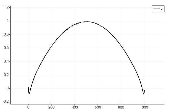
At the inlet of the domain, a parabolic velocity profile was specified to prevent any unnecessary numerical stiffness near the walls where a no-slip condition is immediately adjacent to a specified inlet velocity. Thus, a parabolic profile which achieves a velocity of 0 as it approaches the walls is necessary (Figure 8).

Figure 8. A parabolic velocity profile is specified to prevent any issues with numerical stiffness during the optimization/training process

The numerical approach taken to train this model was to use the Adaptive Moment Estimation (Adam) Optimizer and rely upon a modified Fourier architecture. The modified Fourier architecture was selected based on guidance provided in the Modulus documentation and through collaborations with NVIDIA Modulus developers.

In general, a set of conservation laws can be written as follows:

$\label{eq:5} u_t + \mathcal{N}[u] = 0, x \in \Omega, t \in [0,T]$

Here, $u$ is the solution of the nonlinear partial differential equations (PDEs) over the spatial domain $\Omega$ and time domain $[0,T]$ . The nonlinear differential operator $\mathcal{N}$ is dependent upon the specific conservation law being considered, which in this case is the Navier-Stokes equations. A residual of the following form is used in the Modulus work and is the function that is minimized through the Adam optimizer:

$\label{eq:6} L_{residual} = \frac{1}{N_u}\sum_{i=1}^{N_u}|u(t_u^i,x_u^i)-u^i|^2 + \frac{1}{N_f}\sum_{i=1}^{N_f}|f(t_f^i,x_f^i)|^2$

Figure 9 shows the result of minimizing this residual for the 2D nozzle problem discussed in this work. This type of loss function residual plot is easily generated for Modulus cases by running TensorBoard. For more information about this tool, see the NVIDIA Modulus User’s Guide.

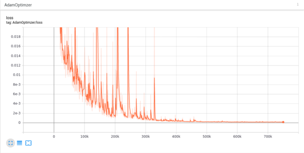
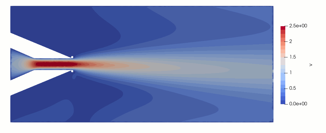
*Figure 9. Adam optimizer displaying the result of minimizing the residual for the 2D nozzle problem*

Figure 10 shows the result velocity distribution across a subset of the radii explored in this work. This animation captures the power of Modulus as an exploratory design tool that can be used to simultaneously train a PINN across a large design space.

Animation of the velocity field of the nozzle after training the Modulus PINN across a range of trailing edge radii. — *Figure 10. The velocity field of the nozzle after training the Modulus PINN across a range of trailing edge radii*

Conclusion

Michael’s application is currently a proof-of-concept written in Python and has been run on one, four, and eight GPUs using their in-house GPU cluster (NVIDIA V100 and NVIDIA A100).

The major distinguishing factor that Michael’s team observed between Modulus and traditional computational physics tools is that it doesn’t rely upon a mesh to discretize the domain and its geometry module provides the flexibility to build parametric features, e.g., edge radii. The scalability of the code on multiple GPUs was another factor that played a role in the Kinetic Vision team’s success in demonstrating Modulus as a viable product design tool.

Michael further elaborated on his experience with Modulus:

“Modulus represents a paradigm change in how some classes of problems are simulated. Scalable compute can be used to explore the entire design space of complex problems, saving hundreds of hours of interactive engineering time to find the optimal result. We have many clients interested in physics modeling as well as machine learning and Modulus is now on our list of technologies that we use to tackle the manufacturing challenges of the Fortune 500.”

For more information, see the Using Physics Informed Neural Networks and Modulus to Accelerate Product Development GTC session. For more information about features and to download the toolkit, see the NVIDIA Modulus product page.